Decomposing the QK circuit with Bilinear Sparse Dictionary Learning

post by keith_wynroe, Lee Sharkey (Lee_Sharkey) · 2024-07-02T13:17:16.352Z · LW · GW · 7 comments

Contents

  Intro and Motivation
  Training Setup
    Step 1: Reconstructing the attention pattern with key- and query-transcoders
      Architecture
      Loss functions
    Step 2: Reducing to Sparse Feature-Pairs with Masking
  Results
    Both features and feature pairs are highly sparse
    Reconstructed attention patterns are highly accurate
        Pattern Reconstruction and Error
    Feature Analysis
      Our unsupervised method identifies Name-Attention features in Name-Mover and Negative Name-Mover Heads
        Name-Moving Key Feature
        Name-Moving Query Feature
      Discovering Novel Feature-Pairs
      Example 1. Pushy Social Media (Layer 10)
        Query Feature
        Key Feature
      Example 2: Date Completion (Layer 10) - Attending from months to numbers which may be the day
        Query Feature
        Key Feature
    Feature Sparsity
      Key- and query-features activate densely
      A dense ‘Attend to BOS’ feature
  Discussion
  Future Work
        ^
        ^
        ^
        ^
        ^
None
7 comments

This work was produced as part of Lee Sharkey's stream in the ML Alignment & Theory Scholars Program - Winter 2023-24 Cohort

Intro and Motivation

Sparse dictionary learning (SDL) has attracted a lot of attention recently as a method for interpreting transformer activations. They demonstrate that model activations can often be explained using a sparsely-activating, overcomplete set of human-interpretable directions. 

However, despite its success for explaining many components, applying SDL to interpretability is relatively nascent and have yet to be applied to some model activations. In particular, intermediate activations of attention blocks have yet to be studied, and provide challenges for standard SDL methods. 

The first challenge is bilinearity: SDL is usually applied to individual vector spaces at individual layers, so we can simply identify features as a direction in activation space. But the QK circuits of transformer attention layers are different: They involve a bilinear form followed by a softmax. Although simply applying sparse encoders to the keys and queries^[1] could certainly help us understand the “concepts” being used by a given attention layer, this approach would fail to explain how the query-features and key-features interact bilinearly. We need to understand which keys matter to which queries.

The second challenge is attention-irrelevant variance: A lot of the variance in the attention scores is irrelevant to the attention pattern because it is variance in low scores which are softmaxed to zero; this means that most of the variability in the keys and queries is irrelevant for explaining downstream behaviour^[2]. The standard method of reconstructing keys and queries would therefore waste capacity on what is effectively functionally irrelevant noise.

To tackle these two problems (bilinearity and attention-irrelevant variance), we propose a training setup which only reconstructs the dimensions of the keys and queries that most affect the attention pattern.

Training Setup

Our training process has two steps:

• Step 1: Reconstructing the attention pattern with key- and query- encoder-decoder networks
• Step 2: Finding a condensed set of query-key feature pairs by masking

Step 1: Reconstructing the attention pattern with key- and query-transcoders

Architecture

Our first training step involves training two sparse dictionaries in parallel (one for the keys and one for the queries). The dictionaries both take in the layer-normalized residual stream at a given layer (normalised_resid_pre_i) and each output a [n_head * d_head] vector, representing the flattened keys and queries^[3]. 

 

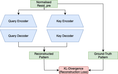
Figure 1: High-level diagram of our training set-up

 

Loss functions

However, rather than penalising the reconstruction loss of the keys and queries explicitly, we can use these keys and queries to reconstruct the original model’s attention pattern. To train the reconstructed attention pattern, we used several different losses:

• KL divergence between the attention pattern (using reconstructed keys and reconstructed queries) and the ground-truth attention pattern produced by the original model.

We also added two auxiliary reconstruction losses both for early-training-run stability, and to ensure our transcoders do not learn to reconstruct the keys and queries with an arbitrary rotation applied (since this would still produce the same attention scores and patterns):

• KL divergence between the attention pattern (using reconstructed keys and the original model’s queries) and the ground-truth attention pattern produced by the original model.
• KL divergence between the attention pattern (using the original models’ keys and the reconstructed queries) and the ground-truth attention pattern produced by the original model.

We also used

• Sparsity regularisation losses on the hidden activations of the transcoders. In our case we used an L_0.5 penalty.

Our architecture and losses allows us to achieve highly-accurate attention pattern reconstruction with dictionary-sizes and L0 values which are smaller than those of the most performant vanilla residual_stream SAEs for the same layers, even when adding the dictionary sizes and L0s of the key and query transcoders together. In this article, we’ll refer to the rows of the encoder weights (residual-stream directions) of the query- and key-transcoders as query- and key-features respectively.

Step 2: Reducing to Sparse Feature-Pairs with Masking

So far this approach does not help us solve the bilinearity issue: We have a compressed representation of queries and keys, but no understanding of which key-features “matter” to which query-features.

Intuitively, we might expect that most query-features do not matter to most key features for most heads, even though they are not totally orthogonal in head-space, since these essentially contribute noise to the attention scores which is effectively irrelevant to post-softmax patterns,

One way of extracting this query-key feature-pair importance data is to take the outer-product of the decoder-weights of the two dictionaries to yield a [d_hidden_Q, d_hidden_K, n_head] “feature_map”.

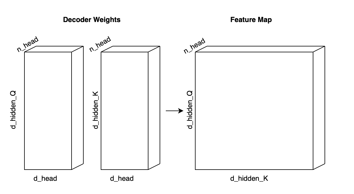
Fig 2. Combining decoder weights to yield a query-key feature importance map

Intuitively, the (i,j,k)-th index of this tensor represents: “If query_feature i is present in the destination residual stream and key_feature j is present in the source residual stream, how much attention score will this contribute to this source-destination pair for head k” (Assuming both features are present in the residual stream with unit norm).

Naively we might hope that we could simply read off the largest values to find the most important feature-pairs. However this would have a couple of issues:

1. No magnitude information: The entries represent the attention-score contribution, but they’re calculated using the unit norm query-features and key-features. If the features typically co-occur in-distribution with very large or small magnitudes, it will be a misleading measure of how important the feature-pair is to attention-pattern reconstruction.
2. No co-occurrence information: Feature-pairs could have high attention contribution not because they are relevant to attention pattern, but because they never co-occur in-distribution. They would also need to co-occur in the right order to be able to influence each other. Indeed, the model might learn to to “pack” non-occurring key and query vectors close to each-other to save space and not introduce interference, making raw similarity a potentially misleading measure.

With these issues in mind, our second step is to train a mask over this query-key-similarity tensor in order to remove (mask) the query-key feature pairs that don’t matter for pattern reconstruction. During this second training process, we calculate attention patterns in a different way. Rather than calculate reconstructed keys and queries, instead we use our expanded query-key-similarity tensor. The attention score between a pair of query, key tokens is calculated as:

acts_Q @ (M * mask) @ acts_K

Where acts_Q, acts_K are the activations of the of the query and key transcoders respectively neurons, and M is the [d_hidden_Q, d_hidden_K, n_head] feature_map given by the outer product of the decoder weights, and the mask is initialised as ones. A bias term is omitted for simplicity^[4].

The loss for this training run is, again, the KL-divergence between the reconstructed pattern and the true pattern, as well as a sparsity penalty (L_0.5 norm) on the mask values. We learn a “reduced” query-key feature map by masking query-key feature pairs for which contribution from their inner product does not affect pattern reconstruction

The final product of this training run is a highly sparse [d_hiddenQ, d_hiddenK, n_head] tensor, where nonzero entries represent only the query-key feature pairs that are important for predicting the attention pattern of a layer, as well as the contribution they make to each heads attention behaviour.

We use our method on layers 2, 6, and 10 of GPT2-small (indexing from 0). We train with two encoder-decoders, with d_hidden 2400 each (compared to a residual stream dimension of 768).

Results

Both features and feature pairs are highly sparse

L0 ranges from 14-20 (per-encoder-decoder). Although this results in a potential feature_map of approximately 69 million entries (2400 * 2400 * d_head), the masking process can ablate between approximately >99.9% of entries, leaving a massively reduced set of query-key feature pairs (between 25,000 - 51,000)^[5] that actually matter for pattern reconstruction. While this number is large, it is well within an order of magnitude of the number of features used by residual stream SAEs for equivalent layers of the same model.

Reconstructed attention patterns are highly accurate

We calculate the performance degradation (in terms of both CE loss and KL-divergence of patched logits to true logits) from substituting our reconstructed pattern for the true pattern at run-time. We compare vs. zero-ablating the pattern as a base-line (although ablation of pattern does not harm model performance that much relative to ablating other components).

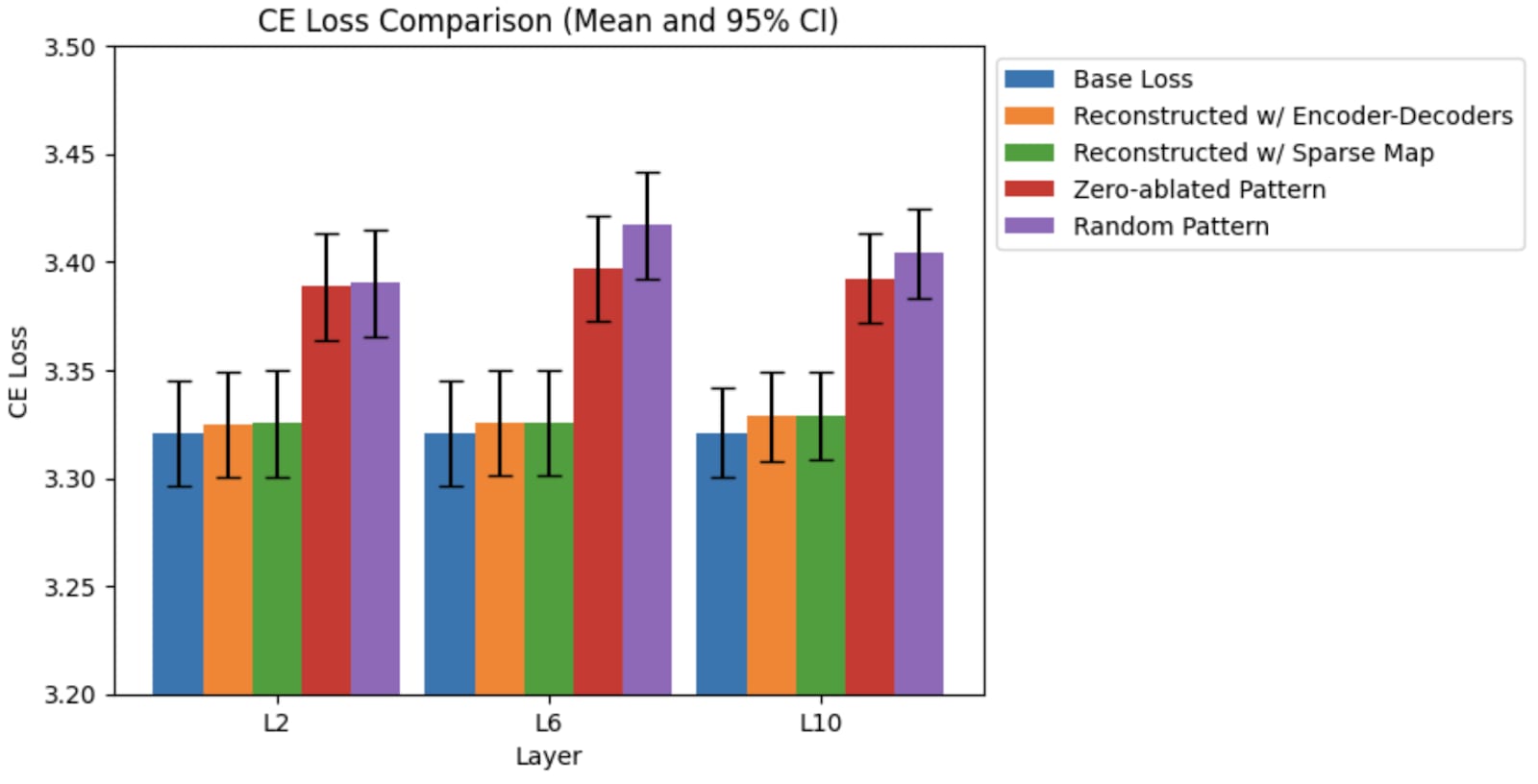
Fig 3. CE Loss for various patching operations relative to base-model loss. We recover almost all performance relative to noising/ablating pattern

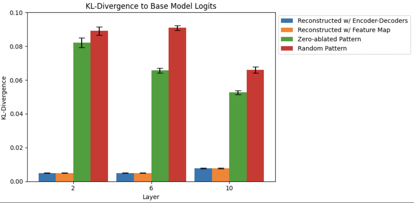
Fig 4. KL-Divergence between logits and base-model logits

Qualitatively, the patterns reconstructed (both with encoder-decoders and with the sparsified feature_map) seem highly accurate, albeit will show some minor discrepancies with higher-temperature softmax contexts. 

Pattern Reconstruction and Error

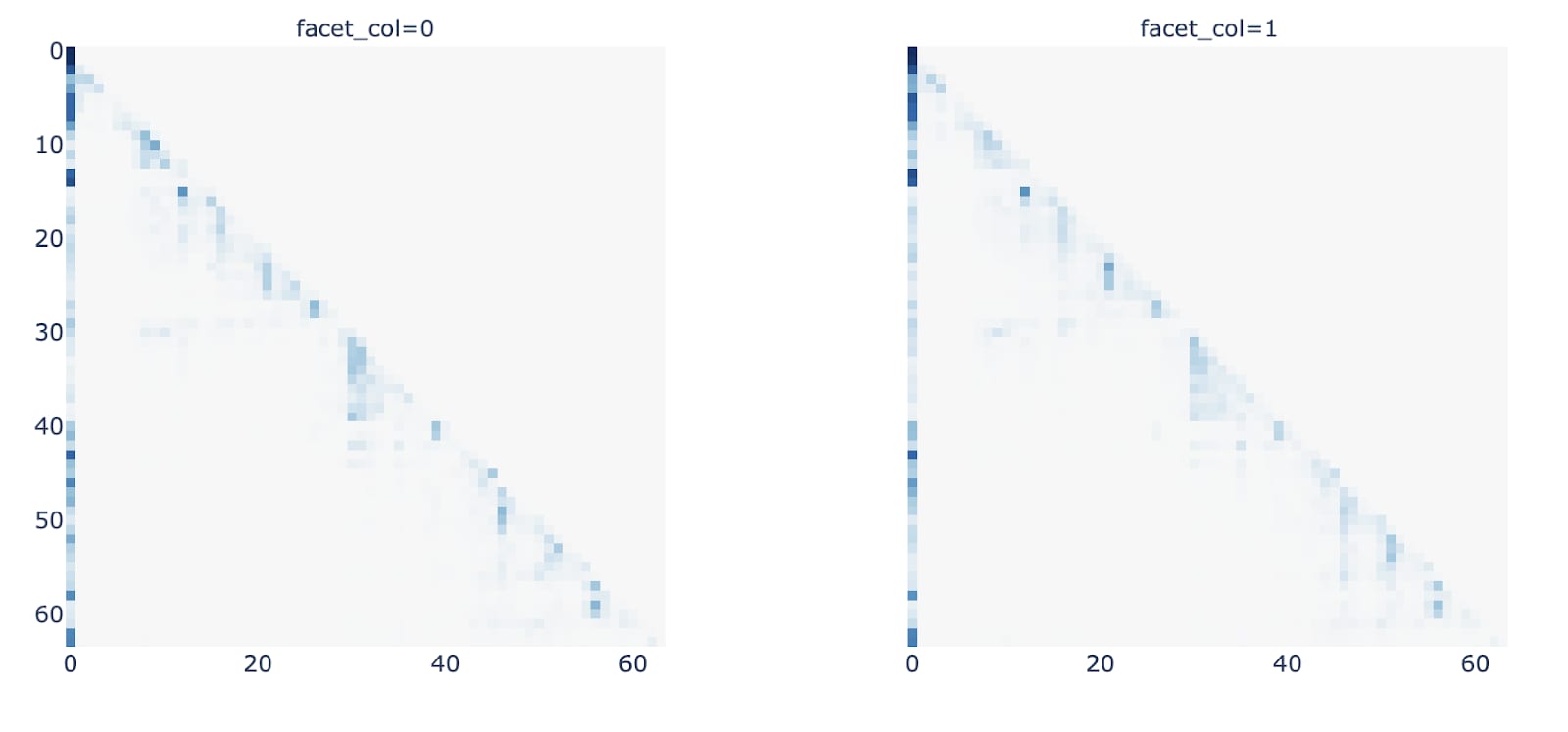
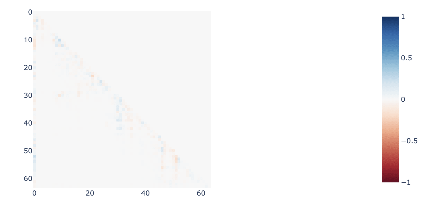
Fig 5. Top displays example pattern reconstruction for L6H0 on a random sequence from openwebtext  (left = True pattern, right = Reconstructed with encoder-decoders). Bottom displays (true_pattern - reconstructed_pattern)

We also look at pattern reconstruction on the smaller IOI templates, for heads involving name-copying and copy-suppression (L10H0, L10H7):

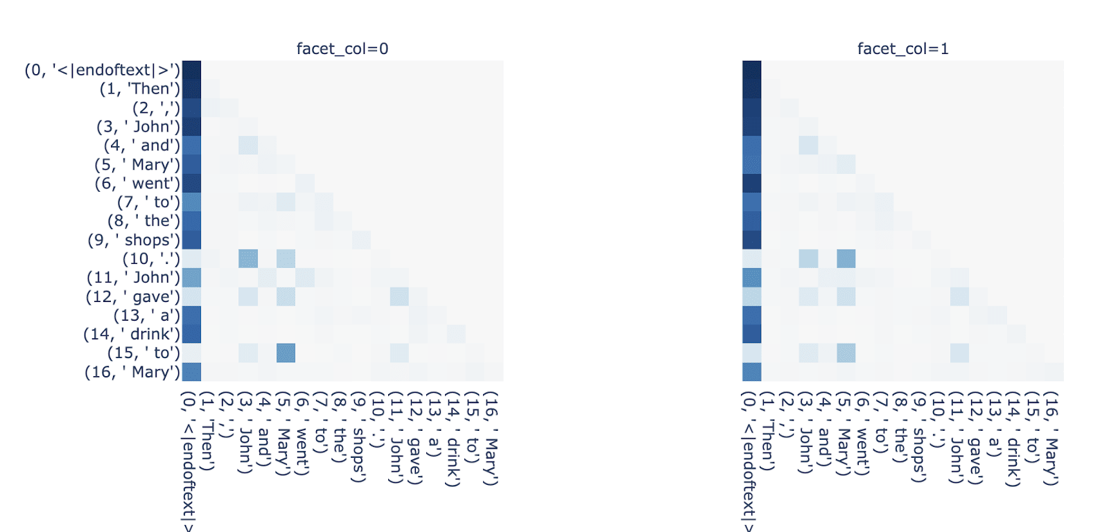
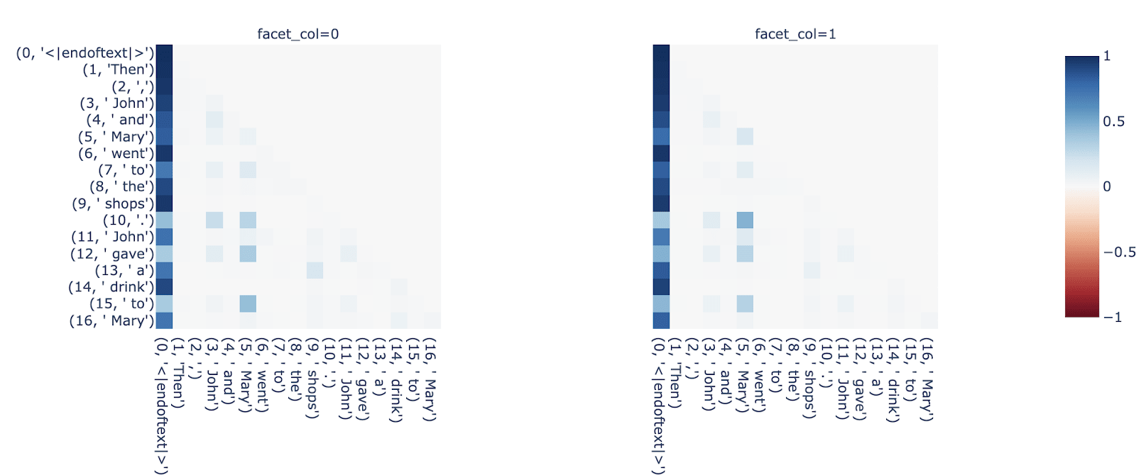
Fig 6. Patterns for L10H0 and L10H7 on IOI template showing attention to names

Feature Analysis

As well as achieving good metrics on reconstruction, we ideally want to identify human-understandable features. As well as examining some randomly sampled features, we looked at features which were active during behaviours that have previously been investigated in circuit-analysis.

Our unsupervised method identifies Name-Attention features in Name-Mover and Negative Name-Mover Heads

Rather than solely relying on “cherry-picked” examples, we wanted to validate our method in a setting where we don’t get to choose the difficulty. We therefore assessed whether our method could reveal the well-understood network components used in the Indirect Object Identification (IOI) task (Wang et al 2022)

In particular, we looked more closely at the name-moving and copy-suppression behaviour found on L10, and looked at the query-key feature pairs in our sparsified feature-map which explained most of the attention to names. For L10H0 and L10H7 (previously identified as a name-mover head and a copy-suppression head respectively), the query-key feature-pair that was most active for both had the following max-activating examples:

Name-Moving Key Feature

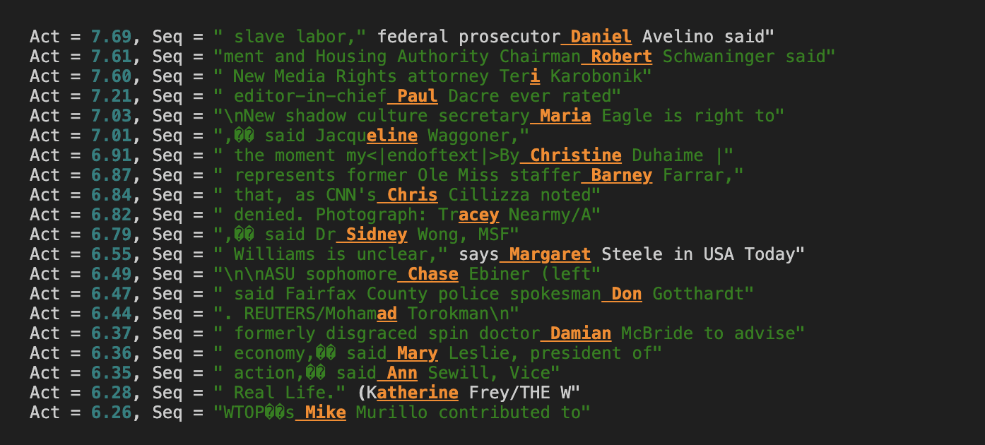
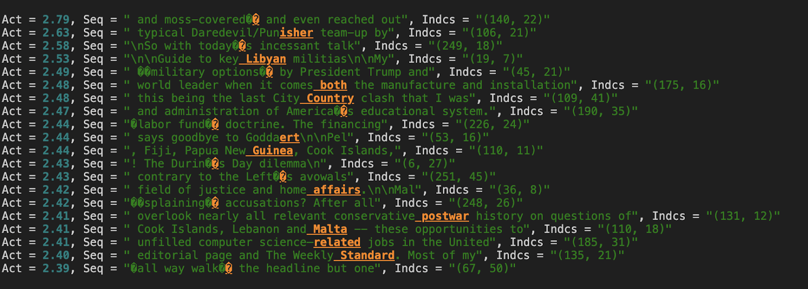
Fig 7. Max activating examples for key-feature, firing on names . The fact that it’s most strongly activating on the last tokens of multi-token names is somewhat confusing, but may have something to do with previous-token behaviour.

Name-Moving Query Feature

Fig 8. Max activating examples for the relevant query-feature. On a first glance this seems quite uninterpretable. But reading more closely these are all contexts where a name would make a lot of sense coming next. Contexts seem to involve multiple individuals, and verbs/prepositions are likely to be followed by names

Interestingly, other query-features seem to attend strongly back to this “name” key feature, such as the following:
 

Second Name-Moving Query Feature

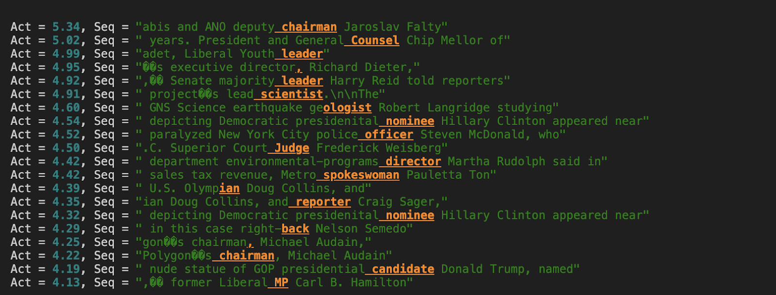
Fig 9. Query feature promoting attention to names. Unlike prepositions/conjunctions, this feature seems to promote attending to names on titles which should be followed by names

This also makes sense as a “name-moving” attention feature, but is clearly a qualitatively distinct “reason” for attending back to names. We believe this could hint towards an explanation for why the model forms so many “redundant” name-mover heads. These feature-pairs do not excite L10H0 equally, i.e. it attends to names more strongly conditional on some of these query features than others. “Name-moving” might then be thought of as actually consisting of multiple distinct tasks distributed among heads, allowing heads to specialise in moving names in some name-moving contexts but performing other work otherwise.

Discovering Novel Feature-Pairs

We also randomly sampled features from our encoder-decoders -  both to check for interpretability of the standalone feature-directions, but more importantly to see whether the feature-pairs identified by the masking process seemed to make sense. An important caveat here is that interpreting features off the basis of max-activating dashboards is error-prone, and it can be easy to find “false-positives”. This is probably doubly-true for interpreting the pairwise relationship between features.

Example 1. Pushy Social Media (Layer 10)

Query Feature

Fig 10: Query Feature max-activating examples: Sign-up/Follow/Subscribe Prompts

Key Feature

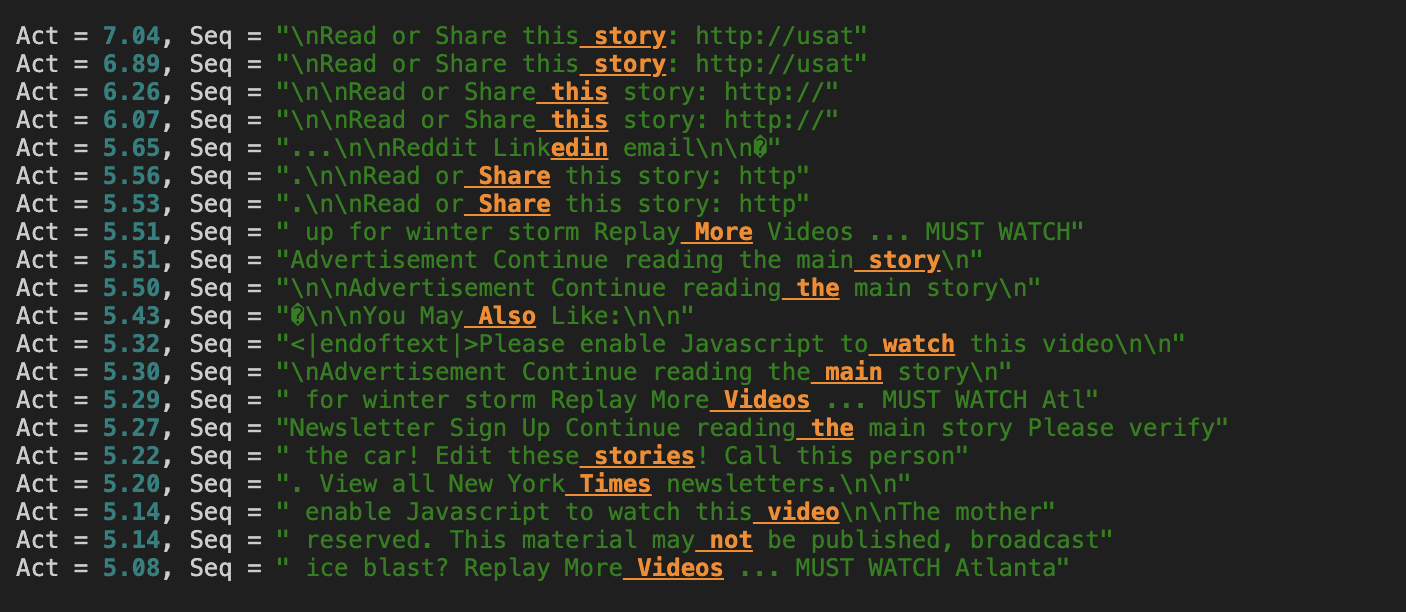
Fig 11: Key Feature with strong post-masking attention contribution to multiple heads. Also firing in the context of social media prompts, but seems to contain contextual clues as to the subject matter (Videos vs. news story etc) that are contextually relevant for completing “Subscribe to…” text.

Example 2: Date Completion (Layer 10) - Attending from months to numbers which may be the day

Query Feature

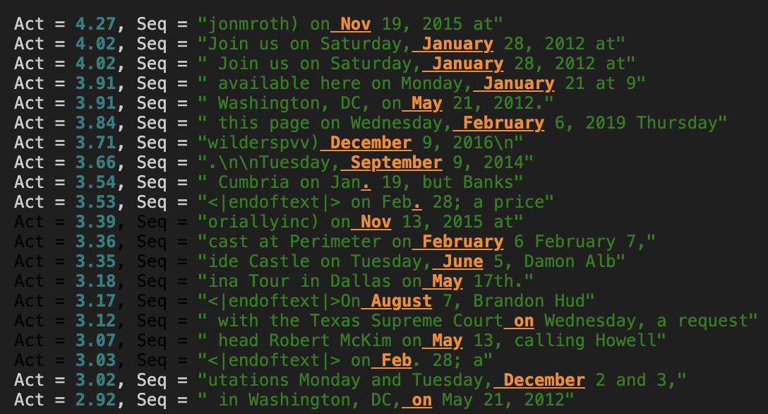
Fig 12: Query-Feature max-activating examples - feature fires on months (which usually precede a number)

Key Feature

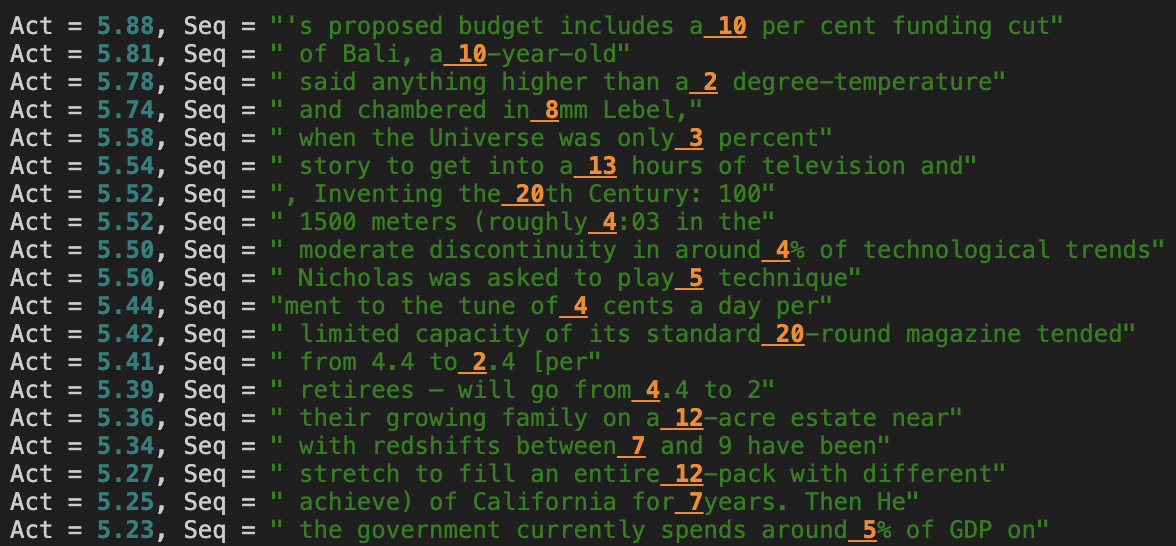
Fig 13: Key-Feature max-activating examples - feature fires on numbers, plausibly used as a naive guess as to the date completion

Feature Sparsity

One quite striking phenomenon in this approach is that, despite starting with very small dictionaries (relative to residual stream SAEs for equivalent layers), and maintaining a low L0, between 80%-95% of features die in both dictionaries. We think this may partly be evidence that in fact QK circuits actually tend to deal with a surprisingly small number of features relative to what a model residual stream has capacity for. But it’s also likely that our transcoders are suboptimally trained. For instance, we have not implemented neuron resampling (Bricken et al 2023). However this phenomenon (and the number of live-features each encoder-decoder settles on) seemed quite robust over a large range of runs and hyperparameter settings, including dictionary size and learning rate, which usually affect this quantity considerably.

Layer	Live Query Features	Live Key Features
2	144	524
6	157	256
10	270	466

Number of live features after training. Both Query and Key encoder-decoders have d_hidden = 2400

The asymmetry in the number of live features in the query and key encoder-decoders also seemed to be consistent, although as clear from the table the exact “ratio” varied from layer-to-layer. 

Key- and query-features activate densely

Finally, the feature density histograms seem intriguing. SDL methods typically assume - and rely upon - the sparsity of feature activations. Our dictionaries yield feature density histograms which are on average significantly denser than those found by residual-stream sparse-autoencoders for the same layers.

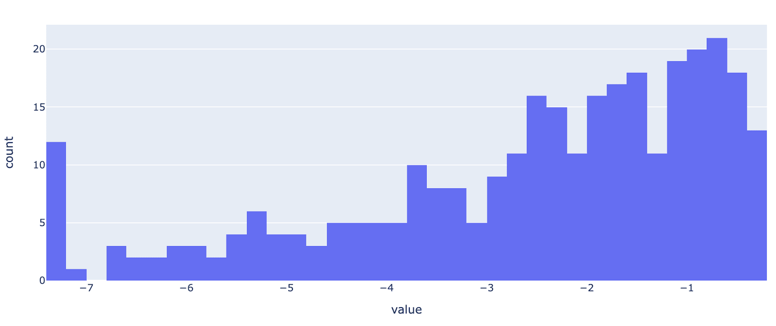
Fig 14: Distribution of log10 frequency for query-encoder-decoder features (after filtering dead neurons)

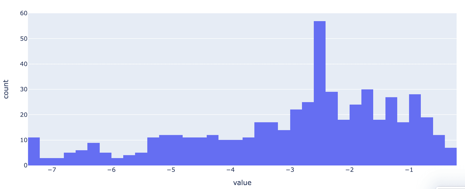
Fig 15: Distribution of log10 frequence for key-encoder-decoder features (after filtering dead neurons)

A dense ‘Attend to BOS’ feature

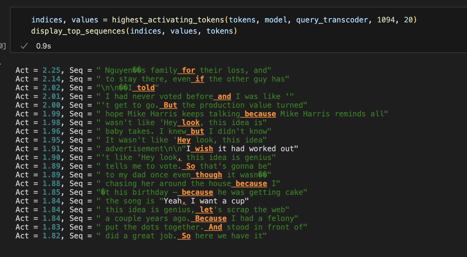
The density of these features seems prima facie worrying; if features are represented as an overcomplete basis but also dense then this might be expected to introduce too much interference. Looking at the max-activating examples of some of these densest query-features also seems confusing:

Fig 15: Fig 16: Dense Query Feature,. Our interpretation: ???

However, we can examine our sparsified feature map to get a sense of what kinds of keys this mysterious dense feature “cares about”. Although there are a few, one of the strongest (which also affects multiple heads) yields the following max-activating examples:
 

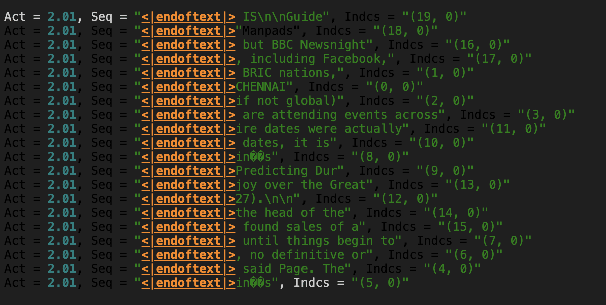
Fig 17: Key feature paid strong attention by multiple heads for the dense query feature. Active solely on BOS tokens

In other words, this dense query-feature seems to prompt heads to want to attend to BOS more strongly! This may suggest that heads’ propensity to attend to BOS as a default attention sink is not purely mediated by biases, but certain query features could act as a “attend to BOS” flag. In these cases it would make sense for these features to be dense, since attending to BOS is a way to turn heads “off”, which is something the network may need to do often.

Discussion

We believe this method illustrates a promising approach to decomposing the QK circuit of  transformers into a manageable set of query-key feature-pairs and their importance to each head. By allowing models to ignore L2 reconstruction loss and instead target pattern reconstruction, we find that we can get highly accurate pattern recovery with a remarkably small number of features, suggesting that a significant fraction of the variance (and by extension, a significant fraction of the features) in the residual stream is effectively irrelevant for a given layer’s attention. Additionally, the fact that the masking process allows us to ablate so many feature-pairs whilst not harming pattern reconstruction suggests very few feature-pairs actually matter for pattern reconstruction.

Attention blocks are a complex and often inscrutable component in transformers, and this method may help to understand their attention behaviour and their subsequent role in circuits. Previously, understanding the role of attention heads via circuit-analysis has been ad-hoc and human-judgement-driven; when a head is identified as playing a role in a circuit, analysis often involves making various edits to the context to gauge what does or does not affect the QK behaviour, and trying to infer what features are being attended between. While our method does not replace the need to perform causal interventions to identify layers/heads of importance in the first place, we believe it provides a more transparent and less ad-hoc way to explain the identified behaviour.

Despite the successful performance and promising results in terms of finding query-key pairs to explain already-understood behaviour, there are several limitations to keep in mind:

Firstly, as mentioned above, we believe the models presented are very likely to be sub-optimally trained. We did not perform exhaustive sweeps for some hyperparameters, and did not implement techniques such as neuron resampling to deal with dead features. It’s therefore possible that when optimally trained, some findings such as the distribution of feature frequency looks different. On the same vein, although we were usually able to find feature-pairs that explained previously-understood behaviour (and most randomly-sampled features seemed to make sense), many features and feature-pairs seemed extremely opaque.

Secondly, although these encoder-decoder networks are significantly smaller than equivalent residual-stream SAEs, we have not trained on other models with enough confidence to get any sense of scaling laws. Although the feature-map ends up significantly reduced, we do ultimately need to start with the fully-expanded [d_hidden_Q, d_hidden_K, n_head] tensor. If the size of optimal encoder-decoder networks for this approach grows too quickly, this could ultimately prove a scaling bottleneck.

Future Work

The results presented here represent relatively preliminary applications to a small number of activations within a single model. One immediate next step will be simply to apply it to a wider range of models and layers - both to help validate the approach and to start building intuition as to the scalability of the method.

Another important avenue for expanding this work is to similarly apply SDL methods to the OV circuit, and to understand the relation between the two. The QK circuit only tells one half of the story when it comes to understanding the role attention heads play in a circuit, and for a fully “end-to-end” understanding of attention behaviour we need an understanding of what OV behaviours these heads perform. However, due to the fact that the OV circuit is neither bilinear nor contains a non-linearity, this should be a much simpler circuit to decompose.

Finally, this approach may lend itself to investigating distributed representation or superposition among heads. Since a feature map represents how interesting a feature pair is to each head, we can see which feature pairs are attended between by one head vs multiple. Although this is far from sufficient for answering these questions, it seems like useful information, and a promising basis from which to start understanding which QK behaviours are better thought of as being performed by multiple heads in parallel vs. single heads.

1. ^{^}

    As a reminder, “query” refers to the current token from which the heads are attending, “keys” refer to the tokens occurring earlier in the context to which the heads are attending

2. ^{^}

    This seems especially important if the residual stream at layer_i stores information not relevant to the attention layer_i (for example, in the case of skip-layer circuits). Unless this information is in the null-space of all heads of layer_i, it will contribute variance to the keys and queries which should nevertheless be able to be safely ignored for the purposes of pattern calculation.

3. ^{^}

    Since the activations being output are different from the input, these are not strictly speaking sparse autoencoders but instead just encoder-decoders, or ‘transcoders’.  

4. ^{^}

    We also need to add a term to capture the interaction effect between the key-features and the query-transcoder bias, but we omit this for simplicity

5. ^{^}

    This number is somewhat inflated due to the fact that most rows correspond to dead-features which can be masked without cost, but even conditioning on live features sparsity is in the range of 80-90%

7 comments

Comments sorted by top scores.