Normalizing Sparse Autoencoders

post by Fengyuan Hu (hufy-dev) · 2024-04-08T06:17:15.536Z · LW · GW · 18 comments

Contents

  TL;DR
  Introduction
  Motivations
  Theoretical Analysis
    Definitions
    The Effect of Input Norms on Feature Suppression
    The Effect of Input Norms on the Inconsistency of L0 Across Layers
  Normalizing SAEs
    Architecture
    Loss
  Experiments 
    Feature Suppression is Suppressed in Normalized SAE
    Normalizing L1 Removes the Correlation Between Input Norm and L0
    L1 Agrees with L0 Better
    Performance Validation
  NSAE Statistics
  Discussion
    Limitations
    Future Work
  Appendix
    Hyperparameters
    Related Work
None
18 comments

TL;DR

Sparse autoencoders (SAEs) presents us a promising direction towards automating mechanistic interpretability, but it not without flaws. One known issue of the original sparse autoencoders is the feature suppression [LW · GW] effect which is caused by the conflict between the $L_2$ and $L_1$ loss and the unit norm constraint on the SAE decoders. This effect in theory will be more evident when we have inputs that have high norms. Another observation is that training SAEs on multiple layers simultaneously results in inconsistent $L_0$ norms for feature activations across layers: in some layers, $L_0$ has scale of  ${10}^2$ , while in some other layers it has a scale of  ${10}^1$. Moreover, the residual states that's inputed to the SAEs for training also have different norms across layers. Hence, I argue that the current SAE architecture is not robust against inputs of varying norms, which is commonly the case in modern LLMs. In this post, I a modified SAE architecture, namely Normalized Sparse Autoencoder (NSAE), and gave a theoretical proof that it will not have the feature suppression problem. I then conducted experiments to verify the effectiveness of the proposed method, which showed that:

1. Feature suppression is suppressed in NSAEs
2. The normalization removed the correlation between layer mean input norm and $L_0$
3. The normalization makes $L_1$ agrees with $L_0$ better

I then further investigated the learned feature dictionaries and identified 3 types of feature vectors: the correction vector, the pillar vector, and the direction vector. I then concluded this post with discussion on the limitations of NSAEs and gave my suggestions on future directions.

Introduction

Training Sparse Autoencoders [LW · GW] (SAEs) on the residual states of pretrained models is a recently proposed method in mechanistic interpretability to tackle the problem of superposition. This method is scalable and unsupervised, making it promising for auto-interpretability research. 

More specifically, a SAE contains an encoder and a decoder. It is trained to generate sparse feature activations from the original residual states of a source model through the encoder, and reconstruct the residual state through a decoder. It is expected that by training the SAE with a large set of activations jointly optimizing for a sparsity loss on the feature activations and a $L_2$ reconstruction loss, the model can learn to decompose residual states into monosemantic feature vectors that are more interpretable.

In this post, I identified a flaw in the original SAE implementation, namely inconsistency of the $L_1$ loss across layers, and proposed a method to mitigate this problem. With the new method, we can significantly decrease the correlation between the norm of the source model's residual activations and the $L_0$ norm of the feature activations, making the training process more robust and controllable. The code is available on GitHub (notice that you should use the dev branch instead of others).

Motivations

Feature suppression [LW · GW] is a known problem for SAEs. It originated from a conflict between the $L_1$ sparsity loss and the $L_2$ reconstruction loss, as the reconstruction's norm is correlated with $L_1$, and the SAE model learns to generate a reconstruction with smaller norm for a better $L_1$ loss. This is not desirable, as we would like the reconstruction to best correspond to the original input activations. Therefore, finding a way to disentangle the input norms from $L_1$ and $L_2$ is beneficial.

Also, in my personal experiments with training SAEs using this implementation from the AI Safety Foundation, I observed an inconsistency of the $L_1$ sparsity loss across layers:

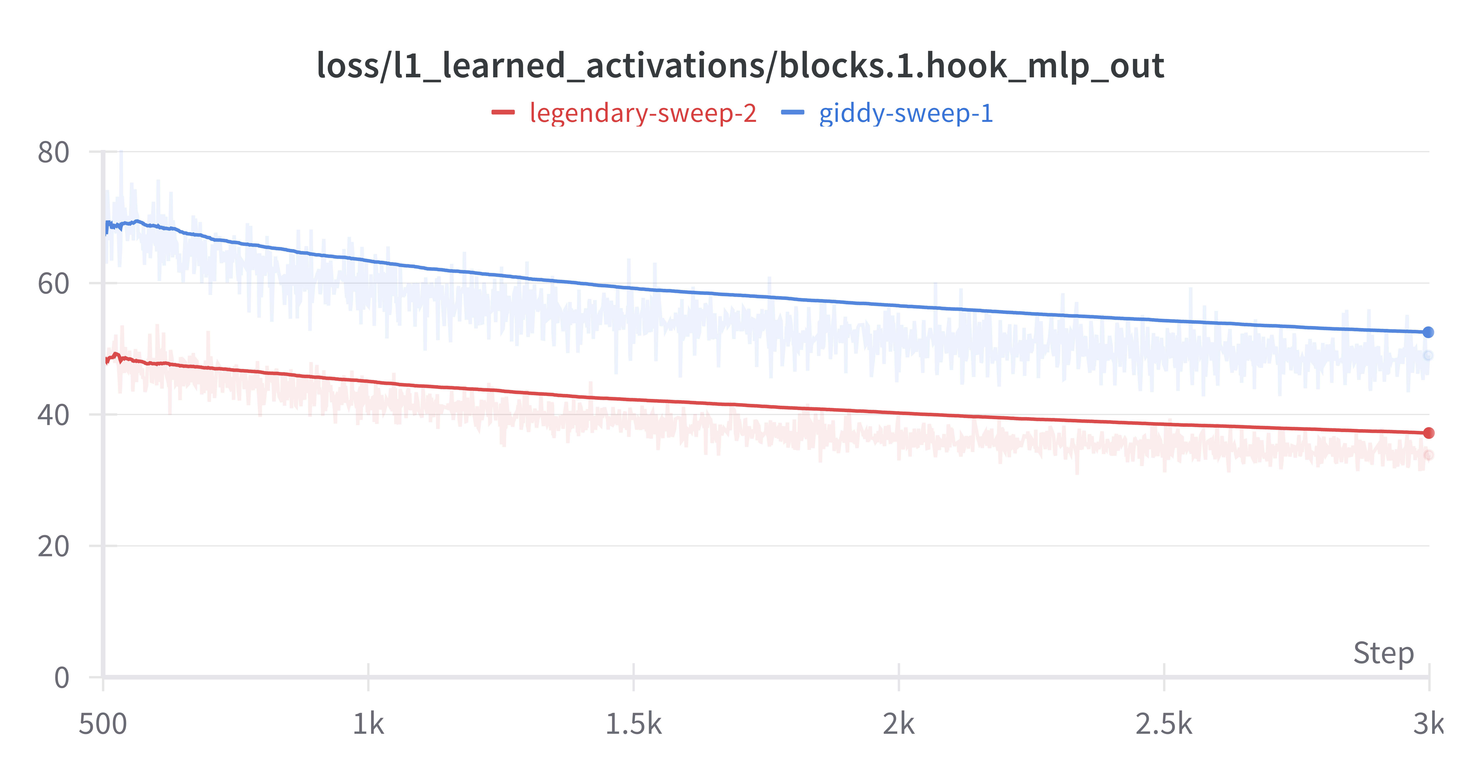
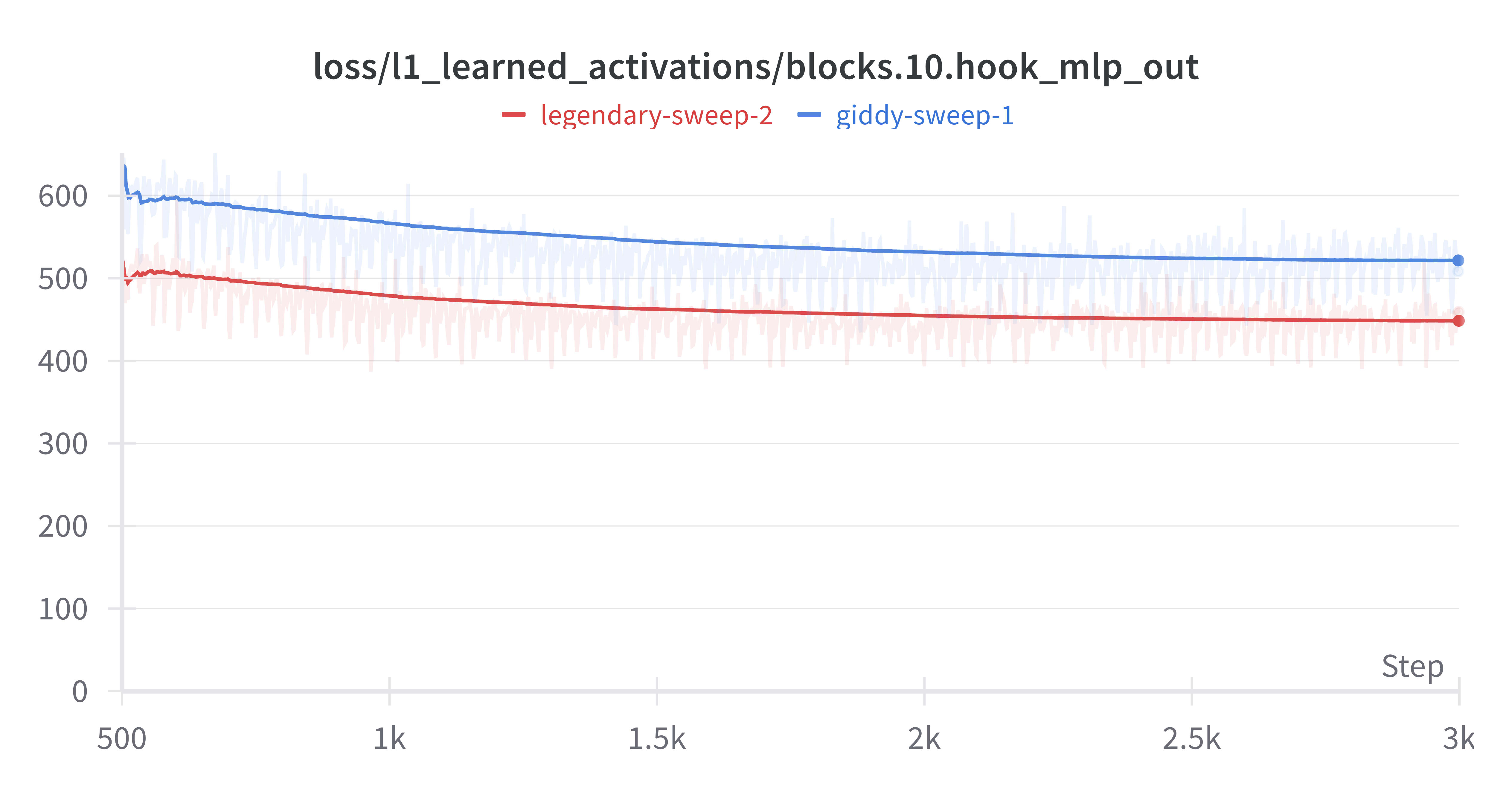
The above two figures are the $L_1$ losses of two different layers from the same training run, but the scale of $L_1$ has a $10\times$ difference.

Moreover, the sparsity measured by $L_0$ is also vastly different across layers:

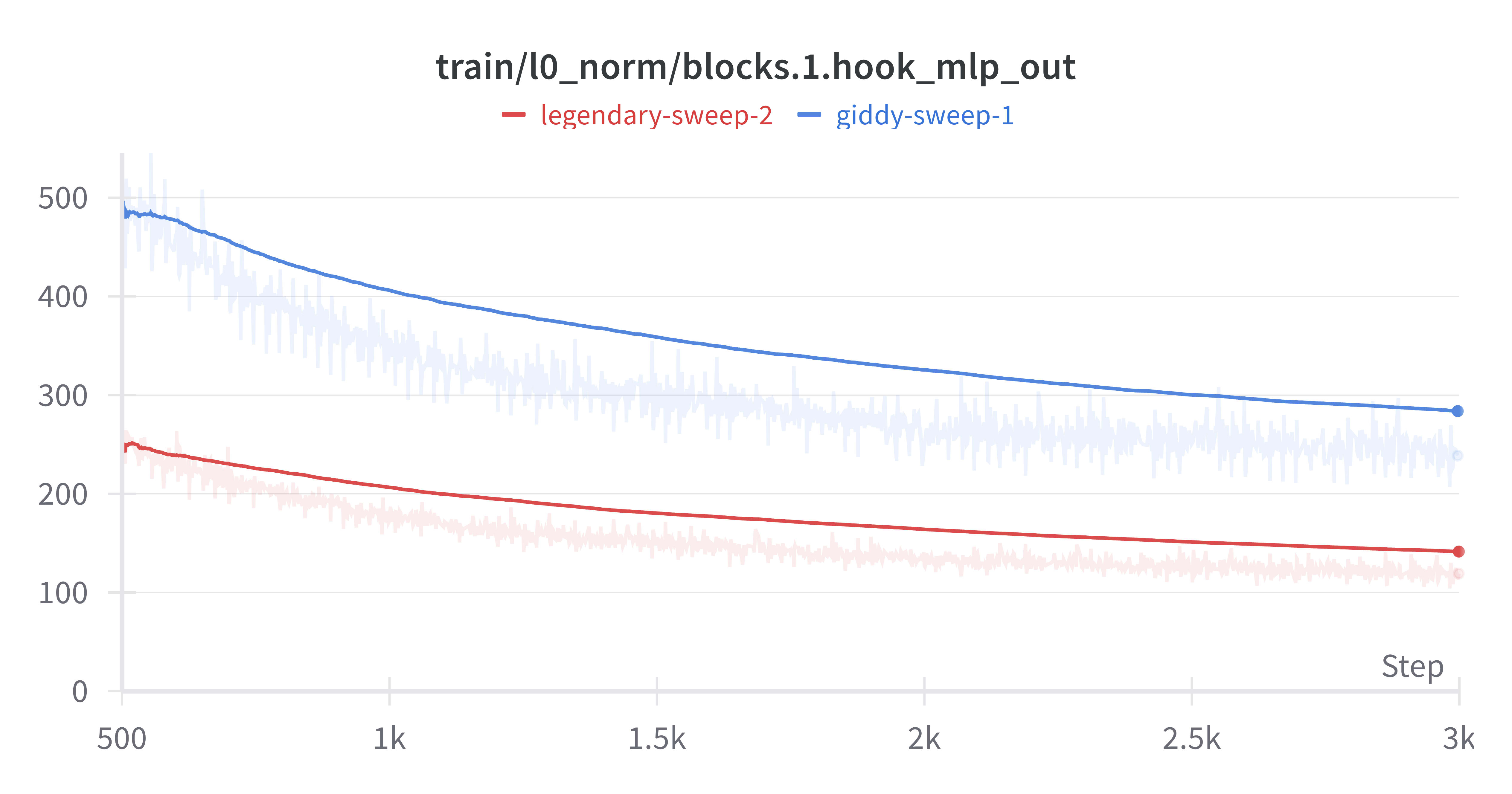
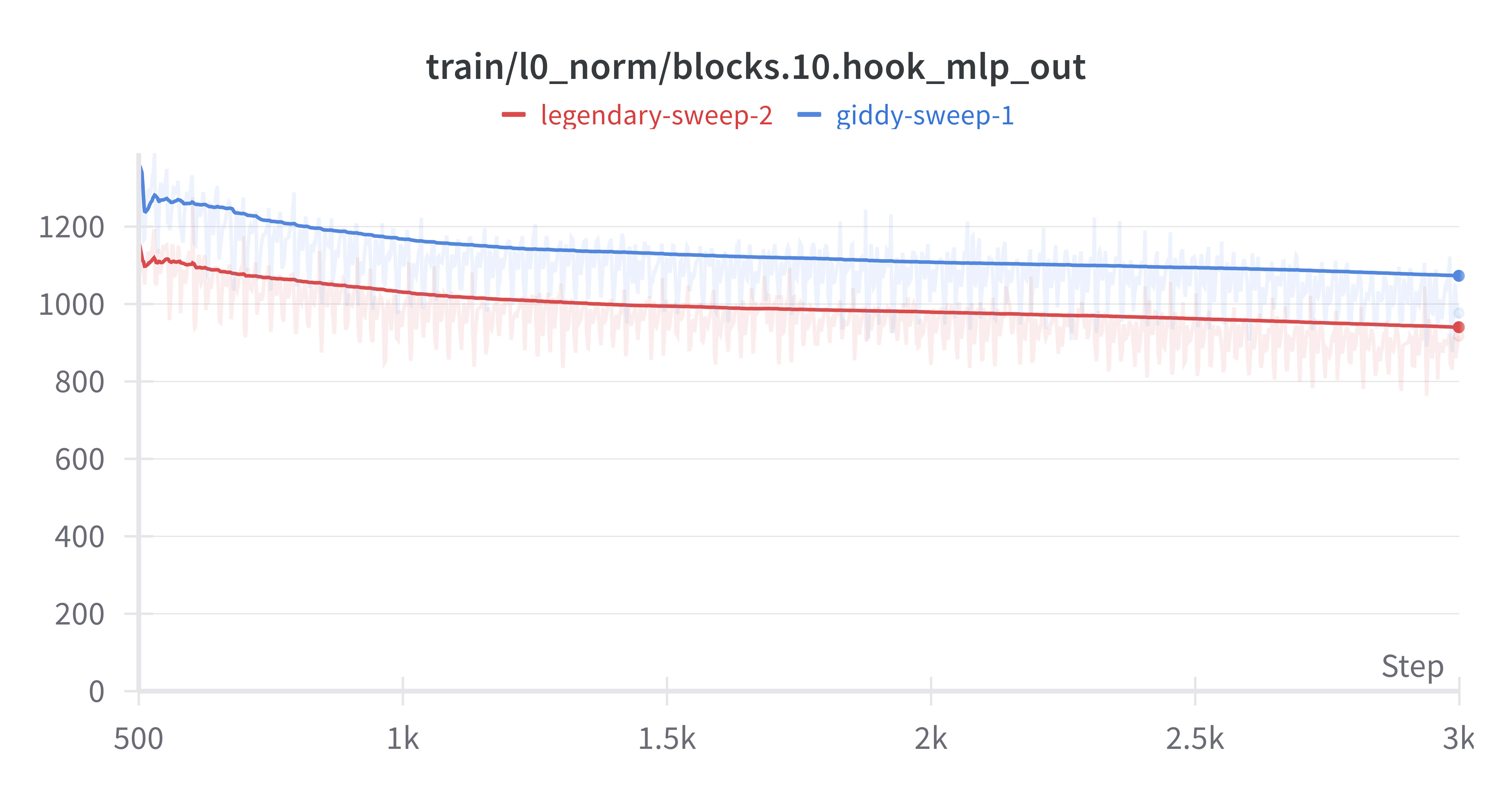
I argue that this is also undesirable, as we introduced the $L_1$ coefficient $\alpha$ in attempt to control the balance between the $L_1$ and $L_2$ loss across layers. Ideally, $\alpha$ should have consistent control across layers, which is not the actual case.

Moreover, there is an inconsistency of the norms of the source model's residual states across layers. We can plot the distribution of residual states^[1] norms in GPT-2 small across layers:

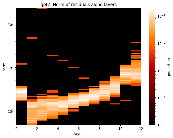
It is obvious that the mean and variance of the norms differ across layers.

This effect is common among LLMs, and we can find similar effects in more recent models like LLaMA-2 and Gemma:

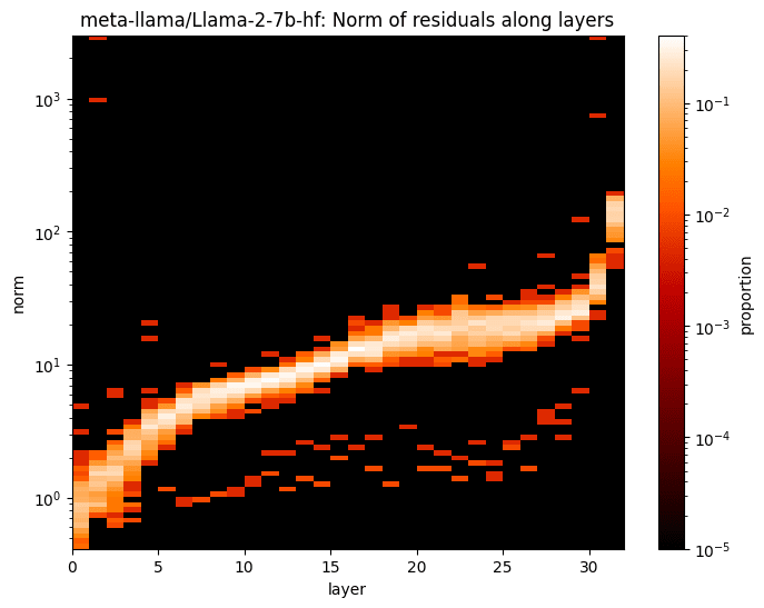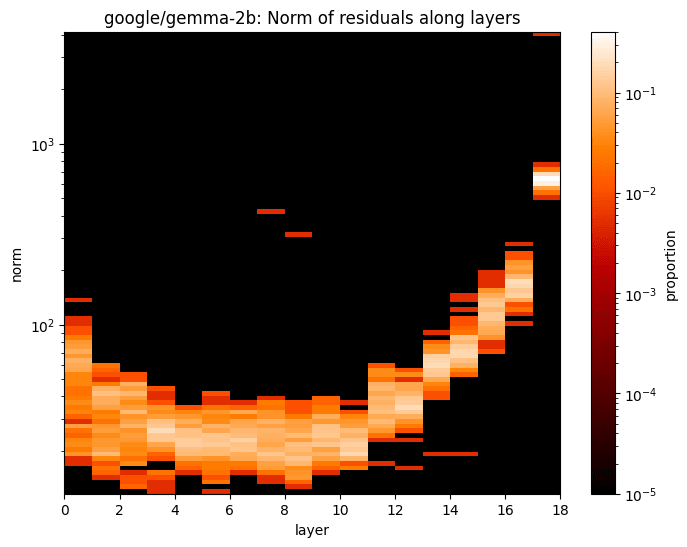This provides some evidence that the inconsistency of input norms might have caused the undesirable behaviors in SAEs. Thus, I will conduct a theoretical analysis in the next section to further illustrate this problem.

Theoretical Analysis

Definitions

With these observations in mind, let's do a theoretical analysis on this loss to see why they might have happened. 

Formally, a SAE can be defined as the following:

$\text{Encoder}\left(x\right)=\text{ReLU}(W_{e}x+b_e)=c$

$\text{Decoder}\left(c\right)=W_{d}c$

$x^{\prime }=\text{SAE}\left(x\right)=\text{Decoder}\left(\text{Encoder}\right(x\left)\right)$

We denote the output of encoder as the feature activation $c$

The loss function for optimization is defined as

$L_1=||c|{|}_1$

$L_2=||x^{\prime }-x|{|}_2$

$L(x^{\prime },x)=\alpha L_1+L_2=\alpha ||c|{|}_1+||x^{\prime }-x|{|}_2$

where the $L_1$ coefficient $\alpha \in R^{+}$ is a hyperparameter of the user's choice and $||\cdot |{|}_k$ is the k-norm of a given vector.

We set another hyperparameter expansion factor $k\in N^{+}$ and denote the source model's residual dimension as $n$. Then we can define $m=kn$ and we have $x,x^{\prime }\in R^n$, $c,b_e\in R^m$, $W_e\in R^{m\times n}$, and $W_d\in R^{n\times m}$.

In the original implementation, the authors constrained the decoder to have unit norm column vectors, so that during the optimization process the model won't minimize the $L_1$ loss by increasing the column norms of the decoder and learn to generate dense feature activation of small $L_1$. This design choice lead to a potential flaw in the method and will be discussed in a later section of this post.

The Effect of Input Norms on Feature Suppression

The authors who identified feature suppression have provided a nice theoretical analysis in the Feature Suppression [LW · GW] section, but for the comprehensiveness of this post, I will conduct a similar analysis using the terms defined in this post.

We first consider the extreme case where an input $x$ has a feature activation $c$ that only has one positive entry $i$, with all other entries equal to 0. Then we have $x^{\prime }=\text{Decoder}\left(c\right)=W_{d}c=c_i{w}_{d,i}$ where $w_{d,i}$ is the $i$-th column vector of $W_d$. Since $W_d$ is column normal, we must have $||x^{\prime }|{|}_2=||c_i{w}_{d,i}|{|}_2=c_i=||c|{|}_1$. 

More generally, I will show that when $||c|{|}_1$ is sparse, we also have $||c|{|}_1\approx ||x^{\prime }|{|}_2$.

Define $I=\{i:c_i\ne 0\}$ the index set of all nonzero entries in the feature activation. Then we assume that the feature vectors in the set $\{w_{d,i}:i\in I\}$ are (almost) mutually orthogonal^[2], which is $\forall i,j\in I,i\ne j,w_{d,i}\cdot w_{d,j}\approx 0$. By the constraint that the decoder have unit norm, which is $\forall i\in I,w_{d,i}\cdot w_{d,i}=1$, we have

$$||x^{\prime }|{|}_2=\sqrt{x^{\prime }\cdot x^{\prime }}=\sqrt{\sum _{i\in I}{c}_i{w}_{d,i}\cdot \sum _{i\in I}{c}_i{w}_{d,i}}=\sqrt{\sum _{i\in I}\sum _{j\in I}{c}_i{c}_j{w}_{d,i}\cdot w_{d,j}}\approx \sqrt{\sum _{i\in I}{c}_i^2}=||c|{|}_2$$

In the case of sparse $c$, we have $||c|{|}_1⪆||c|{|}_2\approx ||x^{\prime }|{|}_2$. 

Then our loss function becomes the following:

$L=\alpha ||x^{\prime }|{|}_2+||x^{\prime }-x|{|}_2$

If we attempt to minimize this loss, there is always a tradeoff between the reconstruction accuracy and the norm of the reconstruction. In most cases, the model will learn to construct $x^{\prime }$ that's close enough to $x$ but slightly smaller than $x$ to achieve low losses in both terms.

The Effect of Input Norms on the Inconsistency of $L_0$ Across Layers

Here, we make the similar assumption that when $||c|{|}_1$ is sparse, we have $||c|{|}_1\approx ||x^{\prime }|{|}_2$.

For the $L_2$ term, we have

$||x^{\prime }-x|{|}_2=||x^{\prime }|{|}_2^2+||x|{|}_2^2-2x^{\prime }\cdot x=||x^{\prime }|{|}_2^2(1+\frac{||x|{|}_2^2}{||x^{\prime }|{|}_2^2}-\frac{2x^{\prime }\cdot x}{||x^{\prime }|{|}_2^2})$

At first glance, this might not be obvious, but if our reconstruction $x^{\prime }$ is similar enough to $x$, we can take $||x^{\prime }|{|}_2\approx ||x|{|}_2$ ^[3]and the equation simplifies to 

$||x^{\prime }-x|{|}_2=||x|{|}_2^2(1+1-2\frac{x^{\prime }\cdot x}{||x|{|}_2\cdot ||x^{\prime }|{|}_2})=2||x|{|}_2^2(1-cos(x^{\prime },x\left)\right)$

Now we can rewrite our loss: 

$L(x^{\prime },x)=\alpha ||x^{\prime }|{|}_2+2||x^{\prime }|{|}_2^2(1-cos(x^{\prime },x\left)\right)$

Notice that, if $1-cos(x^{\prime },x)$ is in a relatively fixed scale, then the first term has a scale of $||x^{\prime }|{|}_2$ while the second term has a scale of $||x^{\prime }|{|}_2^2$. Then , given a fixed $\alpha$, if we have a larger $||x|{|}_2$, the loss term will bias towards the second term, which agrees with the observation I had earlier: the source model's residual states in deeper layers have larger norms than shallower layers, and the $L_1$ loss was significantly higher in deeper layers as the loss was dominated by the larger $L_2$ term.

Normalizing SAEs

After such analysis, it natural for us to ask: is there a way to solve these problems? 

My answer is yes!

Here, I propose an architectural modification to the original SAE architecture, which I have named the Normalized Sparse Autoencoder (NSAE).

Architecture

The modified architecture is defined as the following:

$c=\text{tanh}\left(\text{ReLU}\right(W_{e}x+b_e+ϵ\left)\right)$

$\text{NSAE}\left(x\right)=W_{d}c$

In this definition, $c$ is the new feature activation, and $W_d$ is no longer constrained to unit norm. A Gaussian error term $ϵ$ is introduced to regularize the feature activation, which is sampled from $N(0,\sigma )$ for some hyperparameter $\sigma$.

The introduction of tanh normalizes every entries of $c$ to the range of $[0,1)$. The benefits of doing this are threefolds:

1. This makes $c$ independent of the norm of the input, hence theoretically prevents feature suppression.
2. When the entries of $c$ are in the range of $[0,1)$, $||c|{|}_0$ and $||c|{|}_1$ are much closer, making the $L_1$ loss a more accurate measure of sparsity.
3. The decoder learns features with norms, which can potentially leads to better interpretability as we can now consider both directions and norms. 

The Gaussian noise term is also essential in this architecture. Without it, the model can learn to minimize $L_1$ by learning to map to very small positive values in the feature activation space and learn decoders with extremely large column norms.

To show why adding Gaussian noise solves this problem, I plotted the activation in the following figure:

From the figure, we can see that when the inputs are small, the output of tanh(ReLU) will be relatively sensitive to the input, and adding Gaussian noise can significantly perturb small feature activations. On the contrary, larger inputs to the activation function are much more robust to perturbation, as they all maps to similar values close to $1$. Hence, this perturbation forces the model to learn to generate feature activations that are either strictly 0 or close to 1, which makes $||c|{|}_1$ behave even more like $||c|{|}_0$, especially when we set $\sigma$ to be large.

Loss

We also have to redefine the loss as follows:

$X_i=\{x:x\text{is in the}i\text{-th layer of the input batch}\}$

${\beta }_i=\alpha \cdot \text{mean}(X_i{)}^2$

$L_i(x^{\prime },x)={\beta }_i||c|{|}_1+||x^{\prime }-x|{|}_2$

We introduced the additional step of scaling $\alpha$ by the square of the mean of the input norm of one layer. This is because $||x^{\prime }-x|{|}_2\approx 2||x^{\prime }|{|}_2^2(1-cos(x^{\prime },x\left)\right)$. If we assume that the best an optimizer can do is to achieve a fixed cosine similarity between $x$ and $x^{\prime }$ without the $L_1$ constraint, then we can treat the $(1-cos(x^{\prime },x\left)\right)$ term as a constance, so the $L_2$ loss is of the scale $||x^{\prime }|{|}_2^2\approx ||x|{|}_2^2$, while $||c|{|}_1\approx ||c|{|}_0$ which should be constant across layers. Therefore, we can manually scale the $L_1$ loss to match the scale of the $L_2$ loss. Another way to scale the loss is by using the actual $||x|{|}_2^2$ of the given sample. Theoretically this might cause the model to overfit to inputs of large norms, but for the conciseness of this post, I will leave this problem for future work to investigate, and only use the mean normalization for all the following experiments. 

Experiments 

I trained two groups of SAEs, one baseline and one experiment, on all layers of GPT2, and each group contains 2 training runs trained on $100,000,000$ activations. These four runs used different sets of $L_1$ coefficient and learning rate, and the baseline used the original SAE while the experiment used the normalized SAE. I will use "the experiment group" and "the normalized group" interchangeably. 

Feature Suppression is Suppressed in Normalized SAE

To investigate feature suppression, I added a new verification metric that measures the ratio between the norm of reconstructions and norm of source activations. Here is this measure during training:

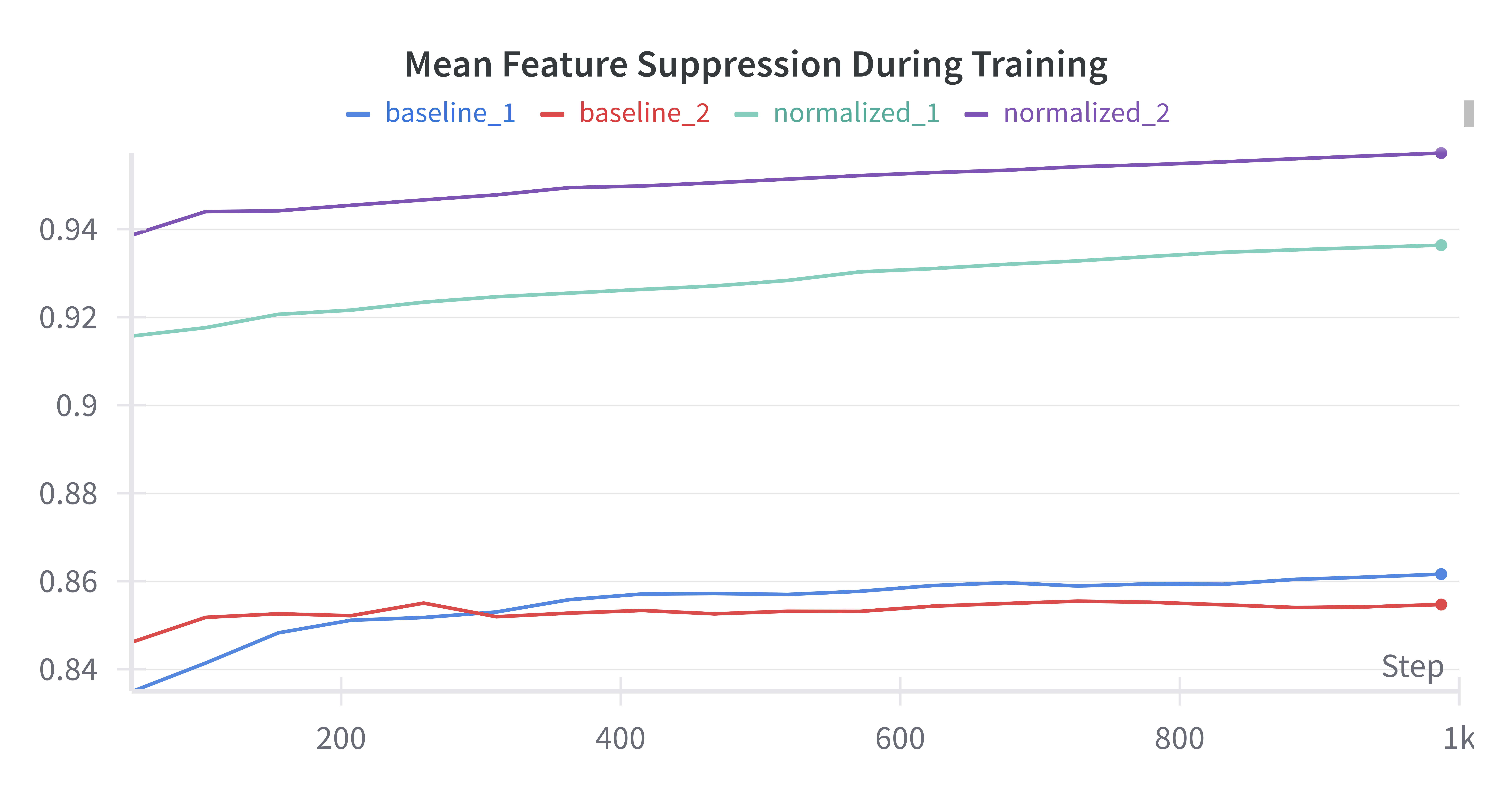
Clearly, the normalized group has significant higher score on feature suppression than the experimental group, and that score is very close to one. Considering the fact that this NSAE didn't fully converge as it only went through 200M training examples, and there is not a sign of this score to flatten, I claim that NSAEs have less to none feature suppression.

Normalizing $L_1$ Removes the Correlation Between Input Norm and $L_0$

To investigate the effect of normalization, I collected the $L_0$ norms of different layers during the end of training and plotted them against the mean input norms of the layer:

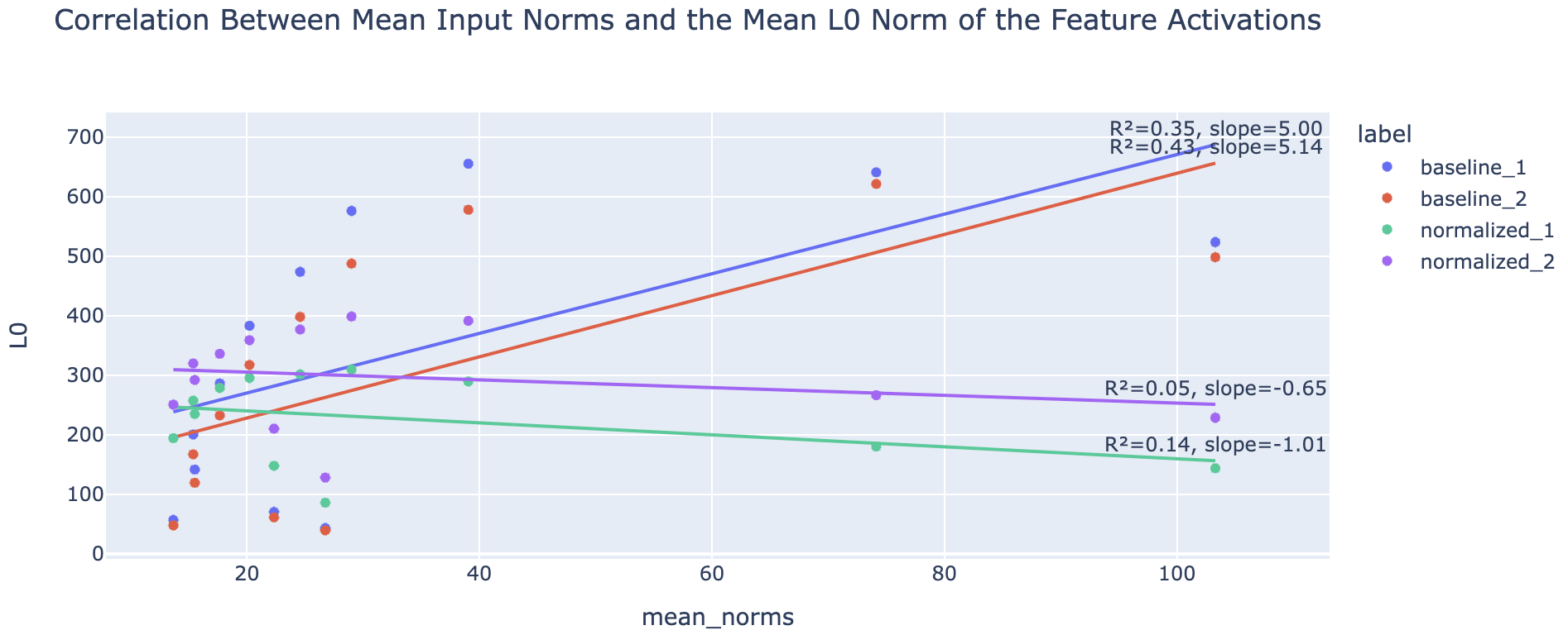
The red and blue datapoints are from the baseline group whereas the cyan and purple datapoints are from the experiment. We can fit lines to these datapoints to find linear relationships between the mean input norm and the mean $L_0$ norm of the feature activations. Although the fitting is not good, the fitted lines still show a rough positive linear correlation between the mean input norm and the feature activation $L_0$ norm in the baseline. In contrast, the two normalized samples did not exhibit a statistical significant positive linear relationship between input norm and $L_0$. 

This linear fit definitely does not look satisfactory, and I further investigated the reasons behind it. I plotted the normalized group's $L_0$ against layer index, and here is what it looks like:

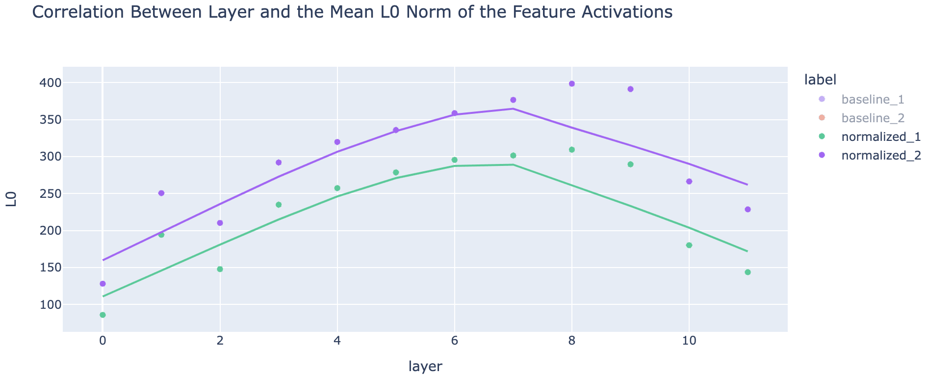
I conjecture that $L_0$ in the normalized group reflects a level of discreteness of the activations of the source model, as it exhibit an increase-then-decrease pattern. In the source model, earlier activations are more discrete as they originated from discrete input embeddings, and as deeper activations might be less discrete as they aggregate information. In the last layers, as the model has to make the next token prediction as accurate as possible, the activations might become more discrete again for better next-token decoding since the decoding layer is discrete. This discreteness might also be positively correlated with the monosemanticity of the activations, as more discrete activations are often more interpretable. I will not verify this conjecture in this post due to length considerations, and I welcome other to study this problem.

$L_1$ Agrees with $L_0$ Better

To investigate the agreement between $L_1$ and $L_0$, I plot the mean $L_0$ and $L_1$ of the feature activations for both groups:

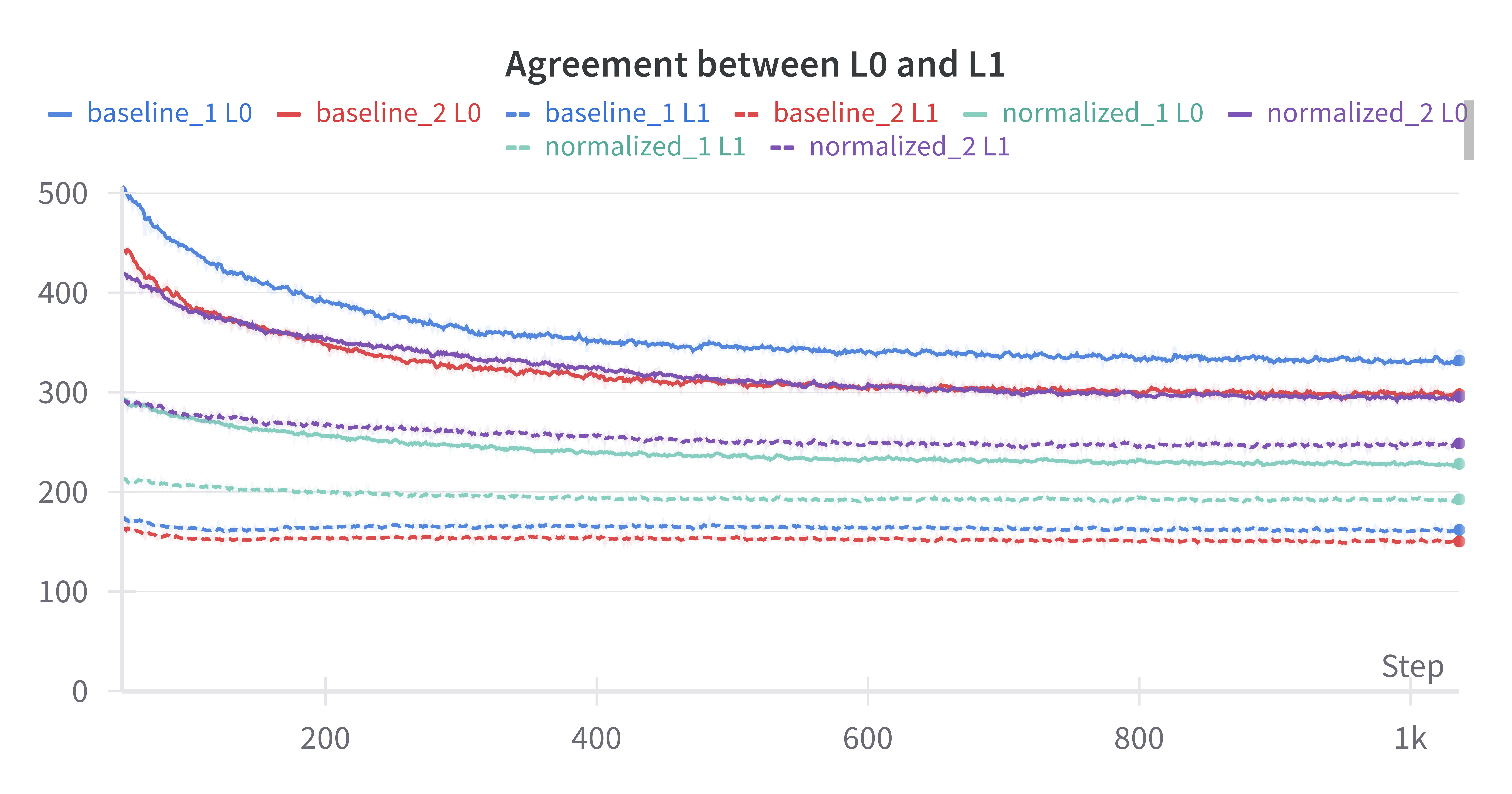
Clearly, the cyan and purple solid lines (which are $L_1$) are much closer to their corresponding dashed lines ($L_0$) than the baselines, indicating better agreement between $L_0$ and $L_1$.

Performance Validation

To validate that the normalization did not heavily impact performance, I present the reconstruction score metric. I first calculate the loss of no intervention, zero intervention (replacing hidden states in one layer with zero vectors), and reconstruction intervention (replacing hidden states in one layer with reconstructed vectors from SAE), and I will denote them as $L_{\text{clean}}$, $L_{\text{zero}}$, and $L_{\text{reconstruction}}$, respectively. Then, the score is calculated by

$S_{\text{reconstruction}}=\frac{L_{\text{zero}}-L_{\text{reconstruction}}}{L_{\text{zero}}-L_{\text{clean}}}$

Since we expect $L_{\text{zero}}$ to be higher than  $L_{\text{clean}}$, and we want  $L_{\text{reconstruction}}$ to be close to  $L_{\text{clean}}$, so higher score is better, and we expect a value close to $1$. The score during training is show below:

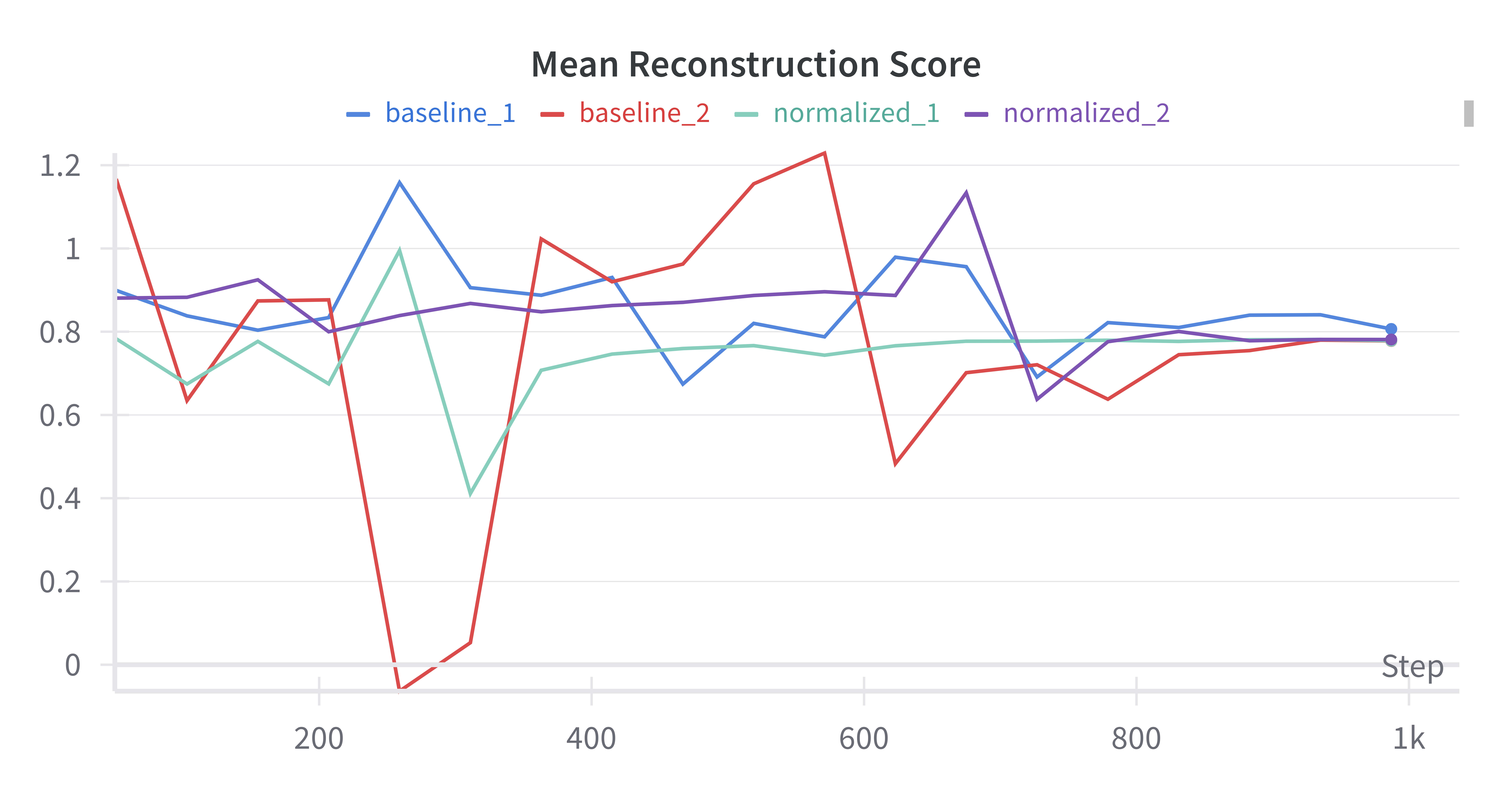
There is no observable difference between the normalized group and the baseline group except that the normalized group's score seems slightly more stable during training, indicating that the normalization did not heavily impact performance but might improved training stability.

Since the mean reconstruction score is heavily impacted by the sparsity of the feature activation, I also compared a layer where the $L_0$ of the baseline and experiment group best agrees with each other:

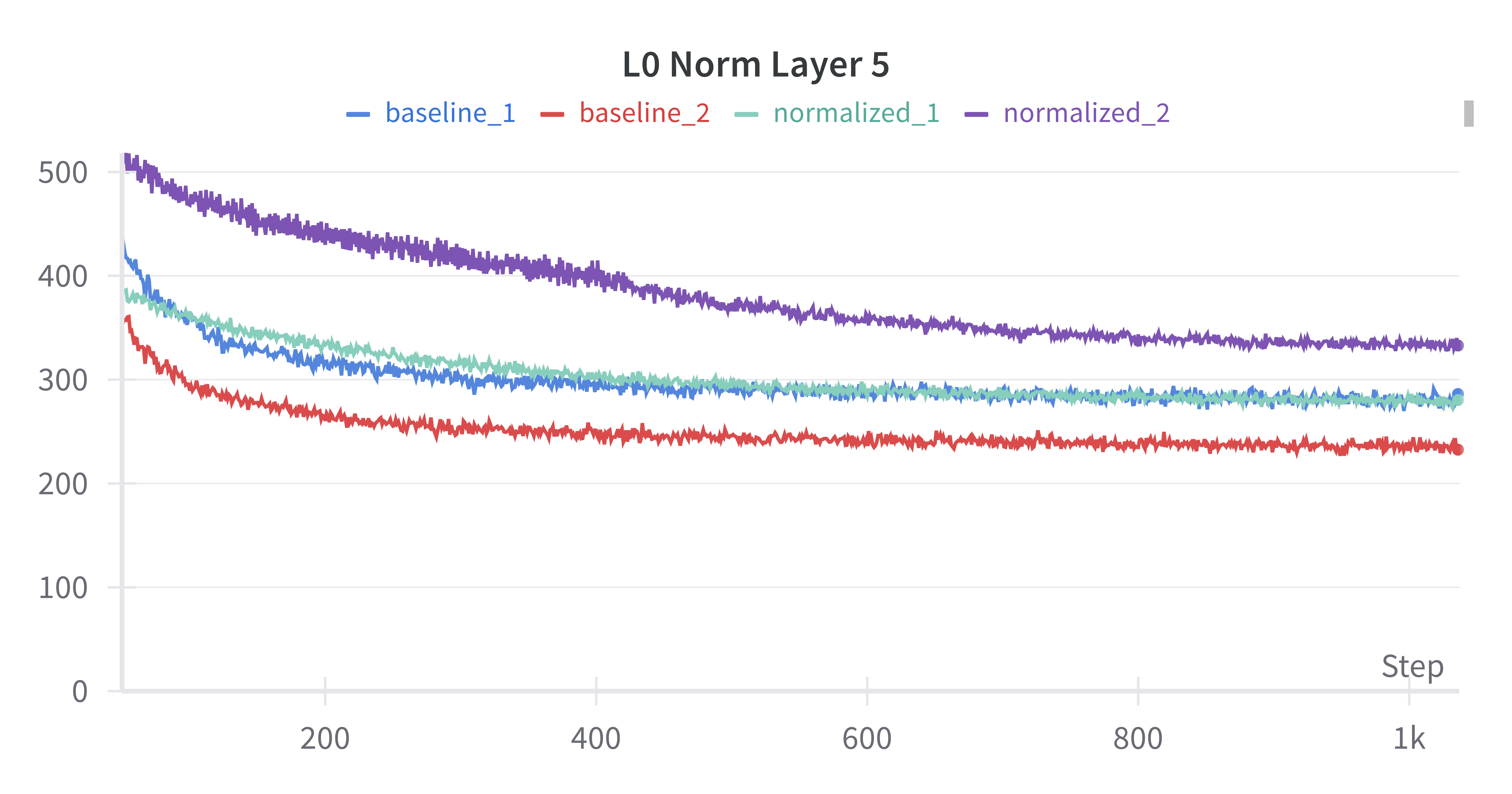
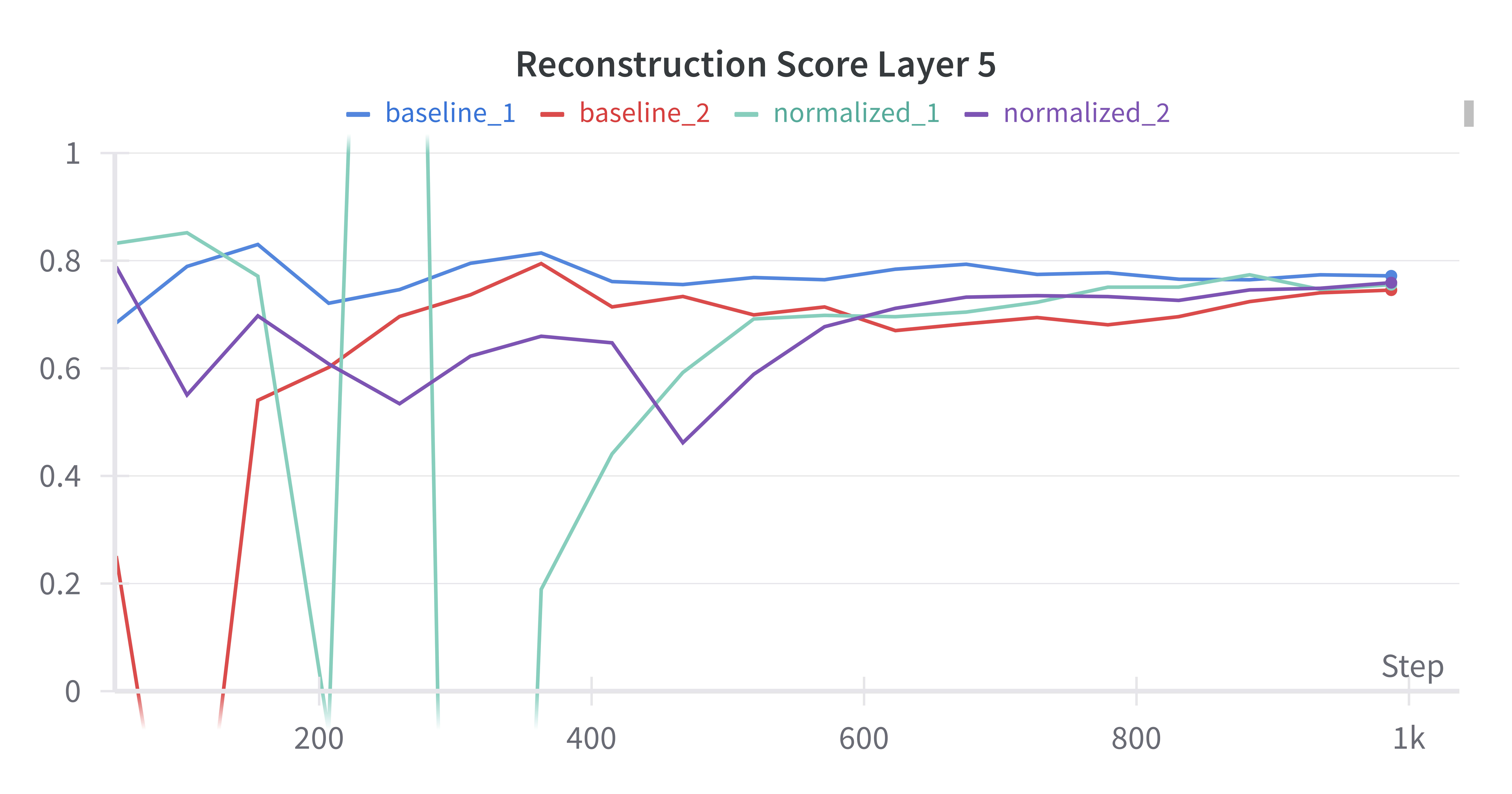
Still, there is not an observable difference between the experimental group and the baseline after convergence. This provided further evidence that the normalization did not have a observable negative impact on the performance of SAEs.

NSAE Statistics

To further investigate what the new SAE has learned, I did some statistical analysis on the NSAE feature dictionary from the first run. For comparison, I used the original SAE trained in the first baseline run.

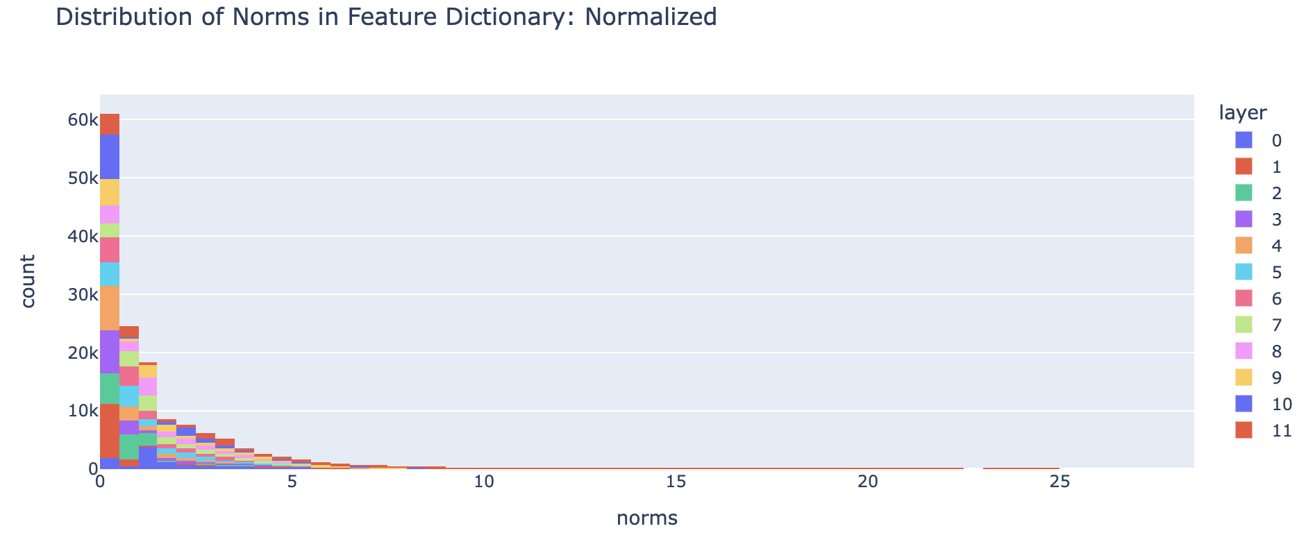
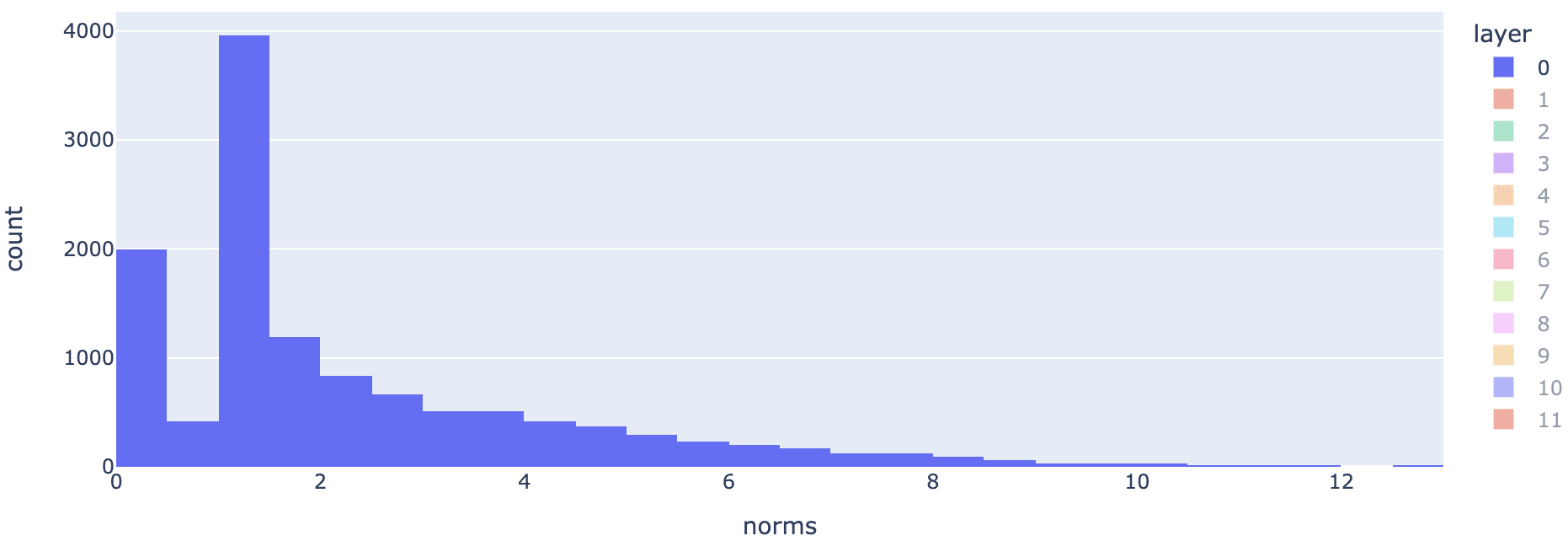
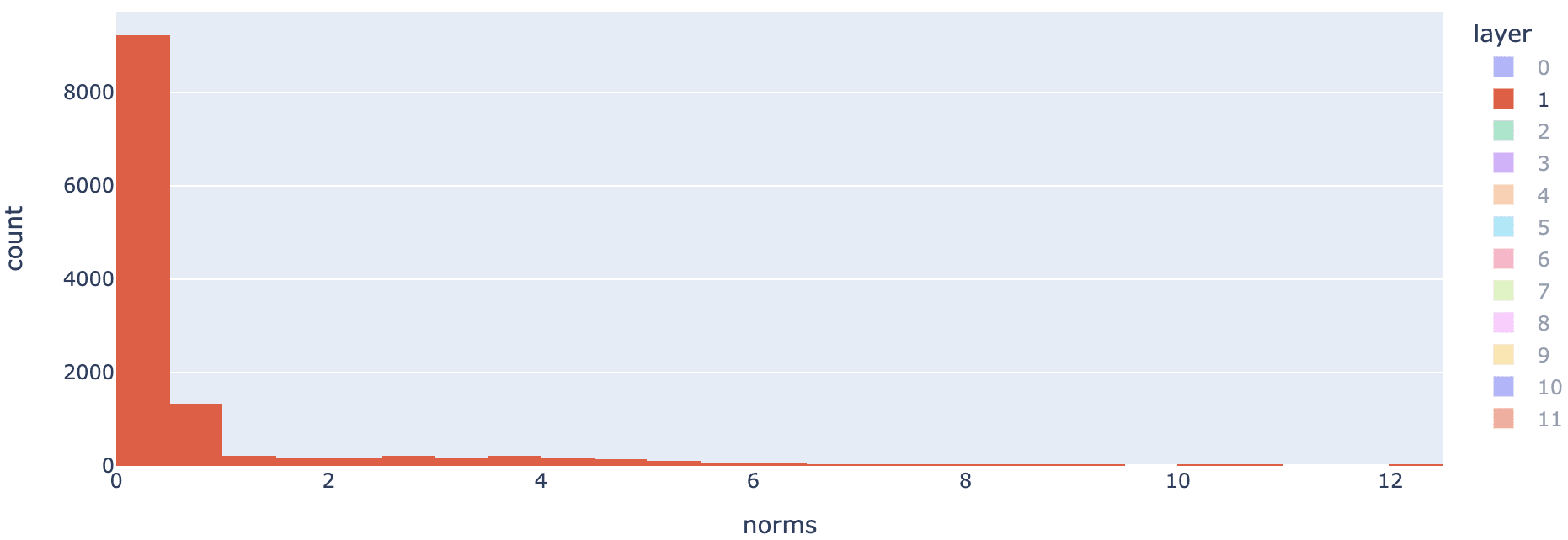
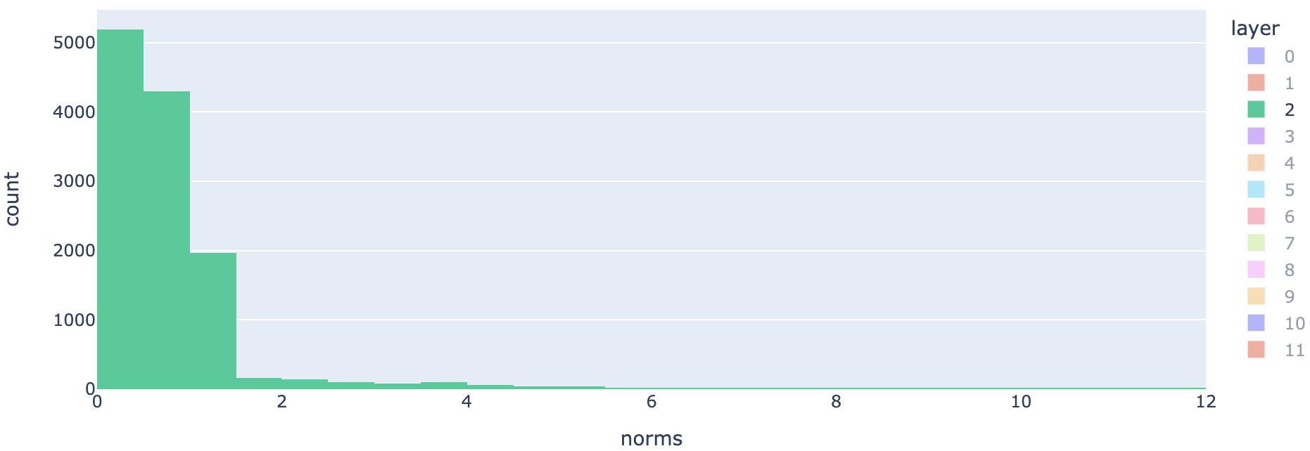
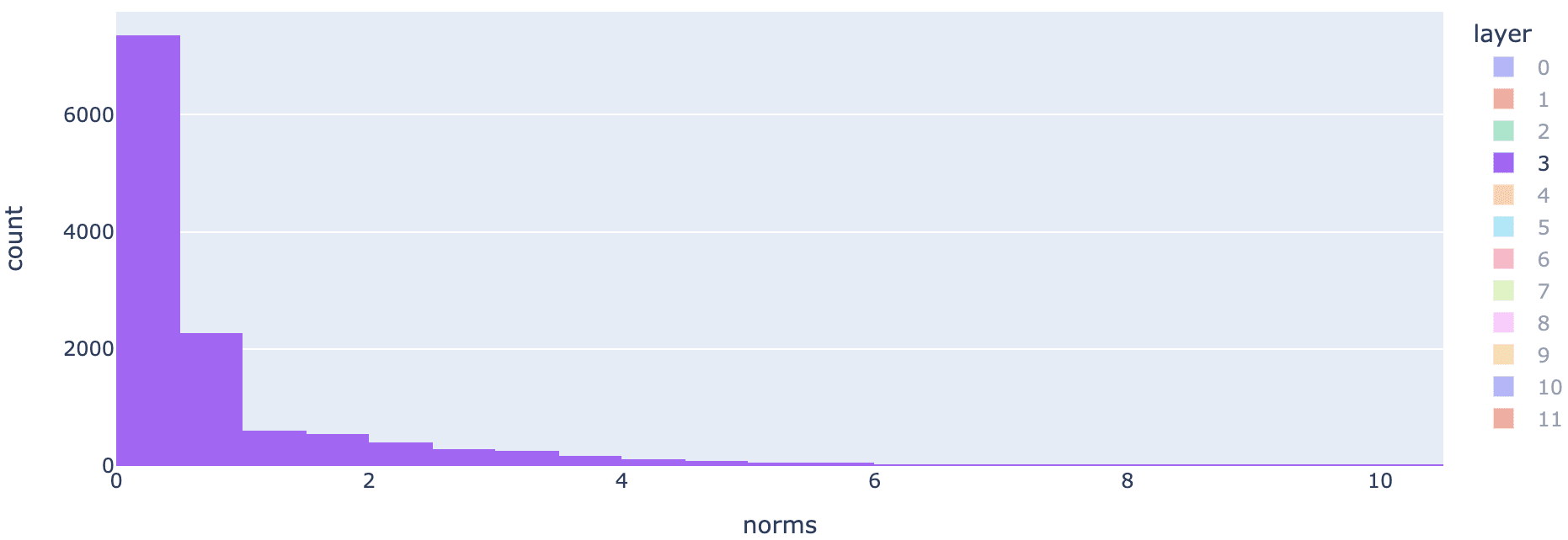
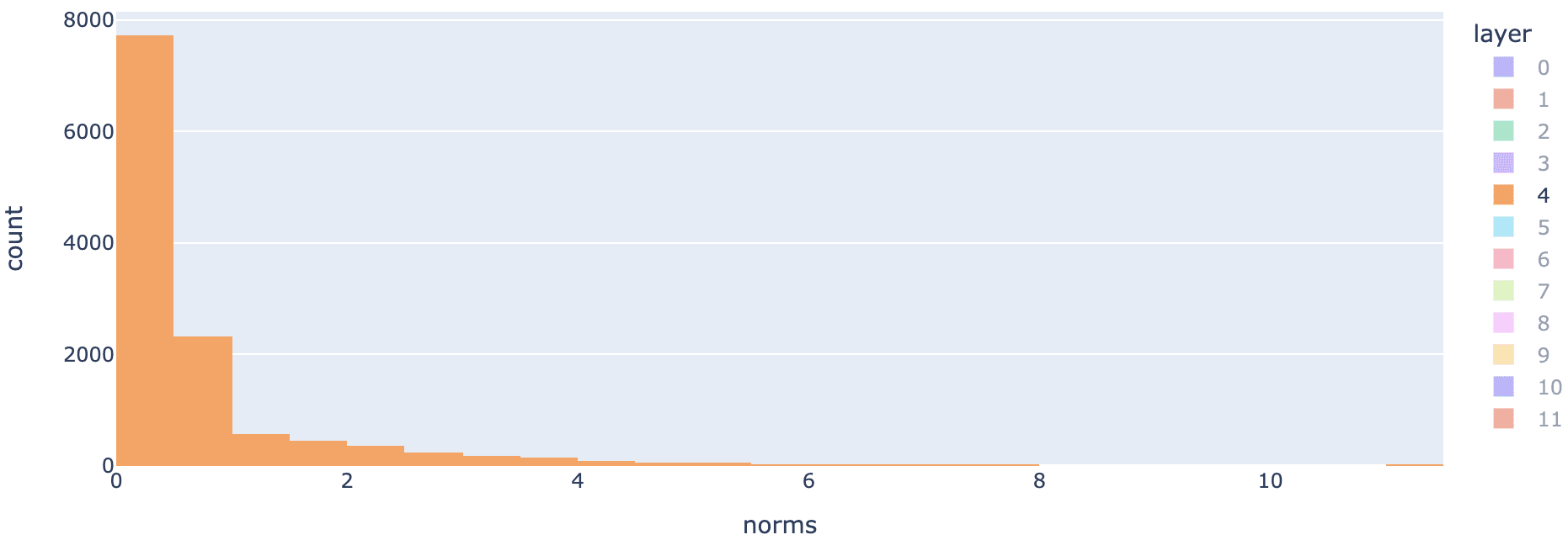
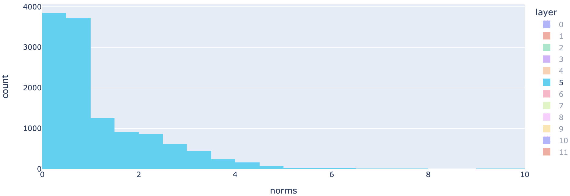
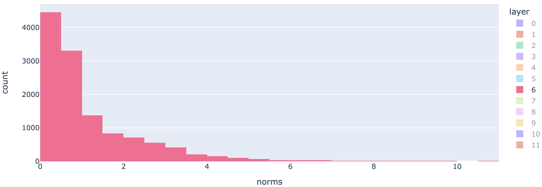
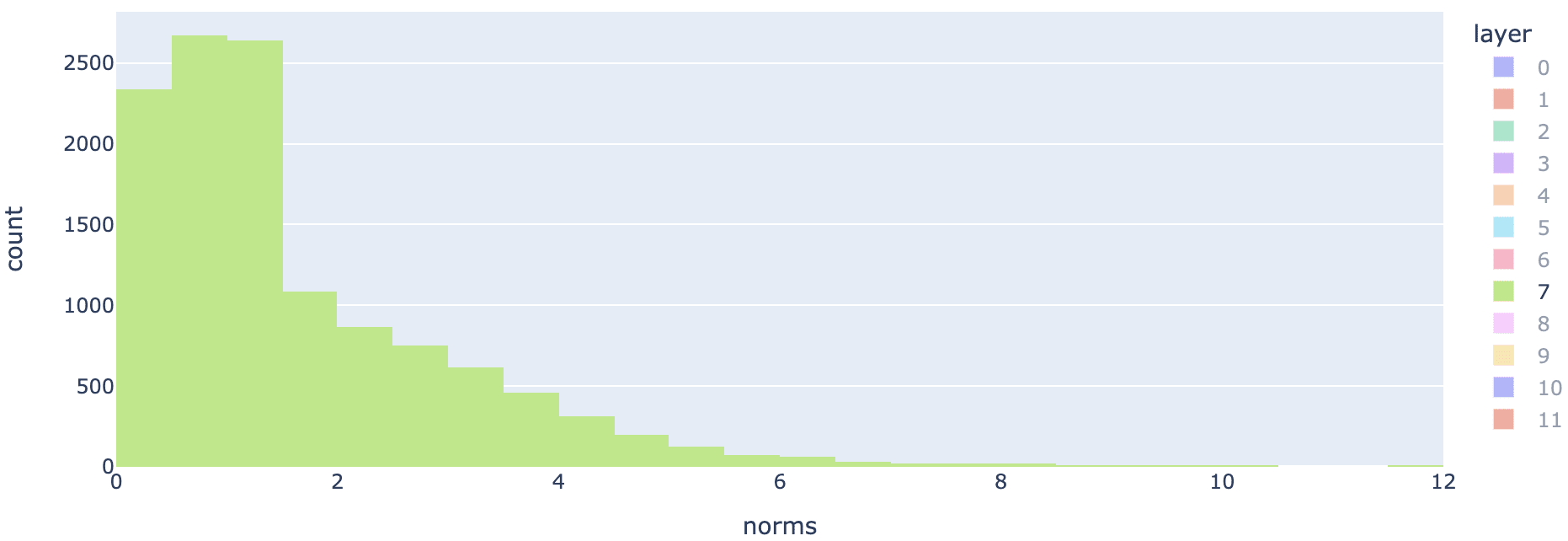
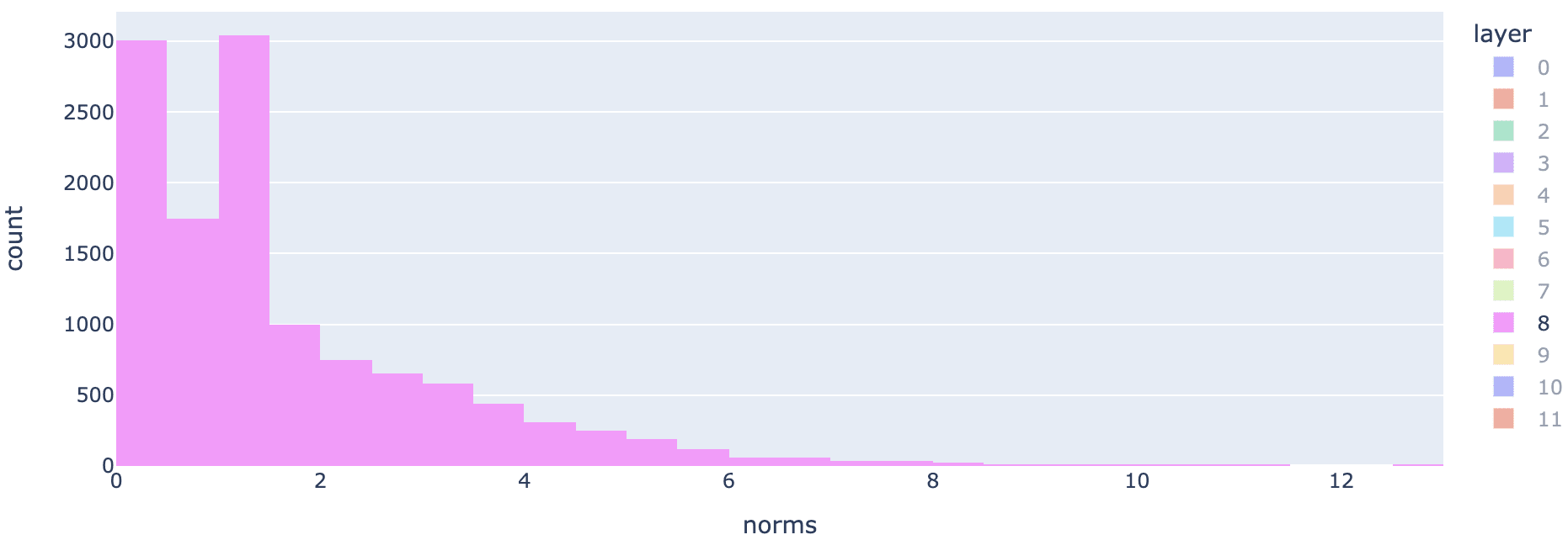
I first analyzed the norm distribution of the feature vectors along the layers:

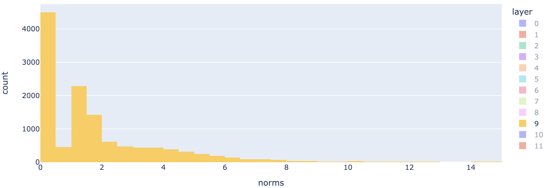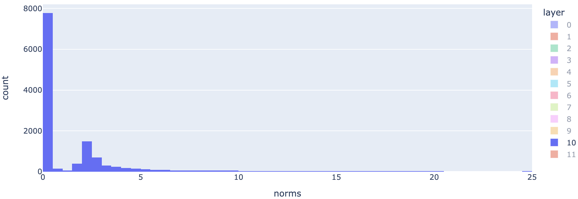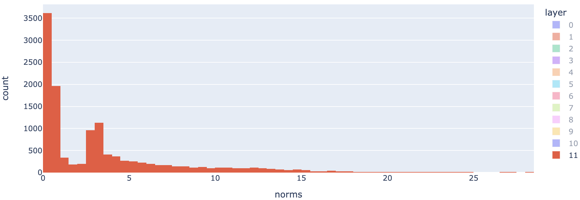Figure 12. Norm distribution histogram of the feature vectors from the NSAE decoder across layers.

Interestingly, a large proportion of feature vectors have norms in the range of $(0,0.5)$, which might indicate that these vectors are small correction vectors that are added to a bigger vector to make the prediction as close as possible. In contrast, I hypothesize that feature vectors of norms that have high mean activation norm should have good interpretability as they represent general directions to the reconstruction. Hence, I will name these vectors as the pillar vectors.

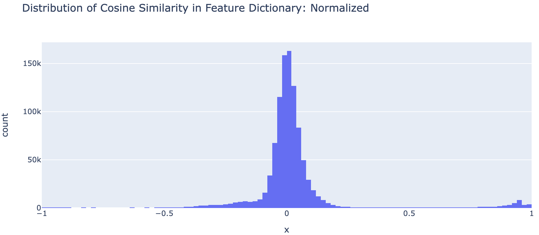
Next, I calculate the distribution of cosine similarity of the feature dictionary:

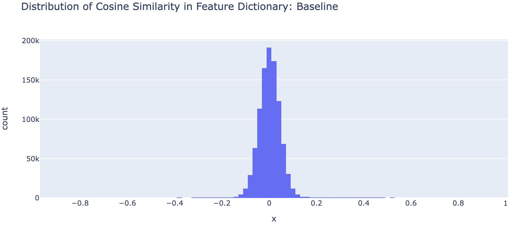Figure 13. Distribution of cosine similarity in the feature dictionary of the NSAE and original SAE, respectively.[4]

From the figure, it's obvious that the cosine similarity distribution of NSAE and SAE are very similar except that in NSAE there are some cosine similarity very close to one. my hypothesis to these vectors is that in NSAE, there are some direction vectors that appears frequently in different norms in the decomposition of source model activations, so that NSAE have to learn these vectors of the same direction in different norms.

A natural question to ask is that: do pillar vectors and direction vectors overlap? To answer this, I picked the top-$100$ vectors (in terms of norm) of each layer from the feature dictionary as a set of pillar vectors and calculated their cosine similarity, and here is the distribution:

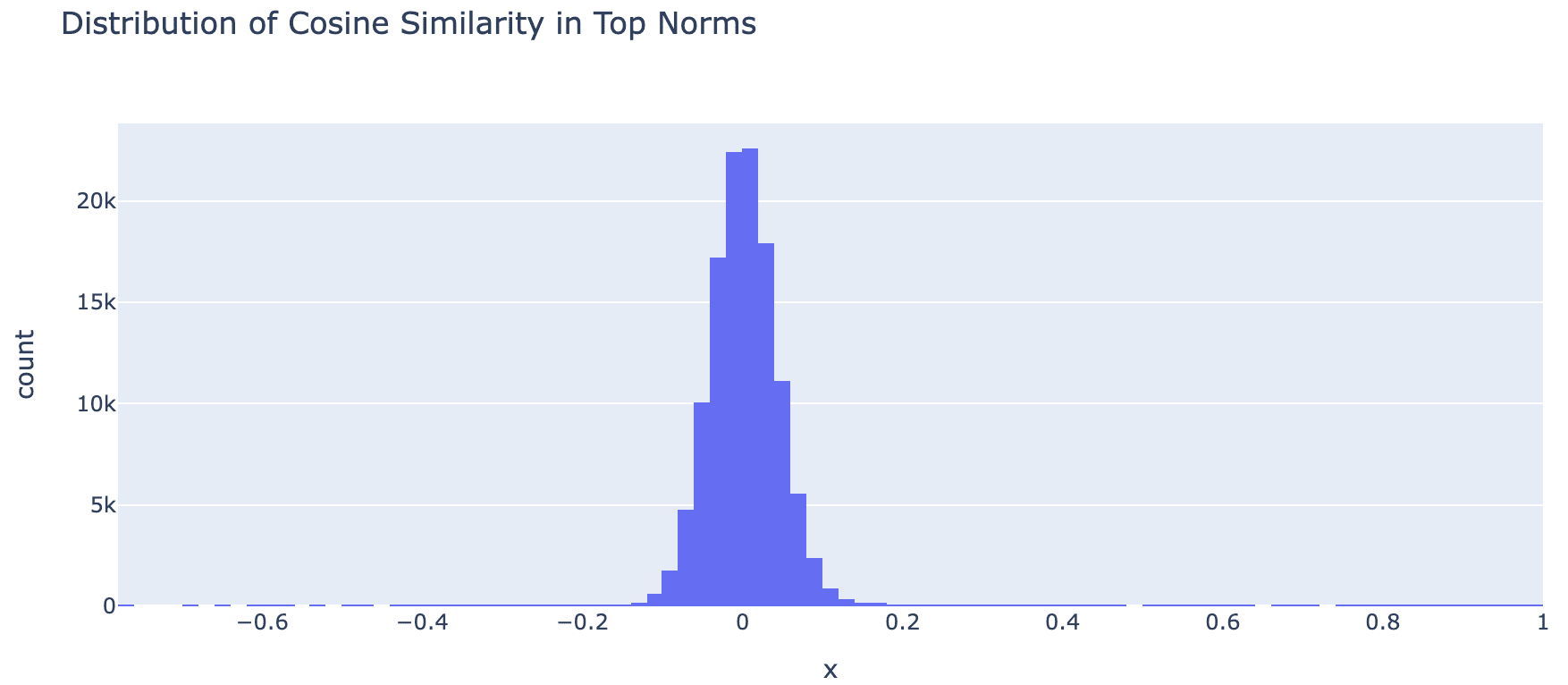
Since the are little to none vectors that have very high cosine similarity, there is minimal overlap between pillar vectors and direction vectors.

As this post is already pretty long, I will leave a more comprehensive analysis on the learned feature dictionary to a future post and conclude this post.

Discussion

Limitations

The normalization did not come without cost. NSAEs generally have slightly higher reconstruction losses compared with the original, and it takes longer for NSAE to converge, as shown in the following figure:

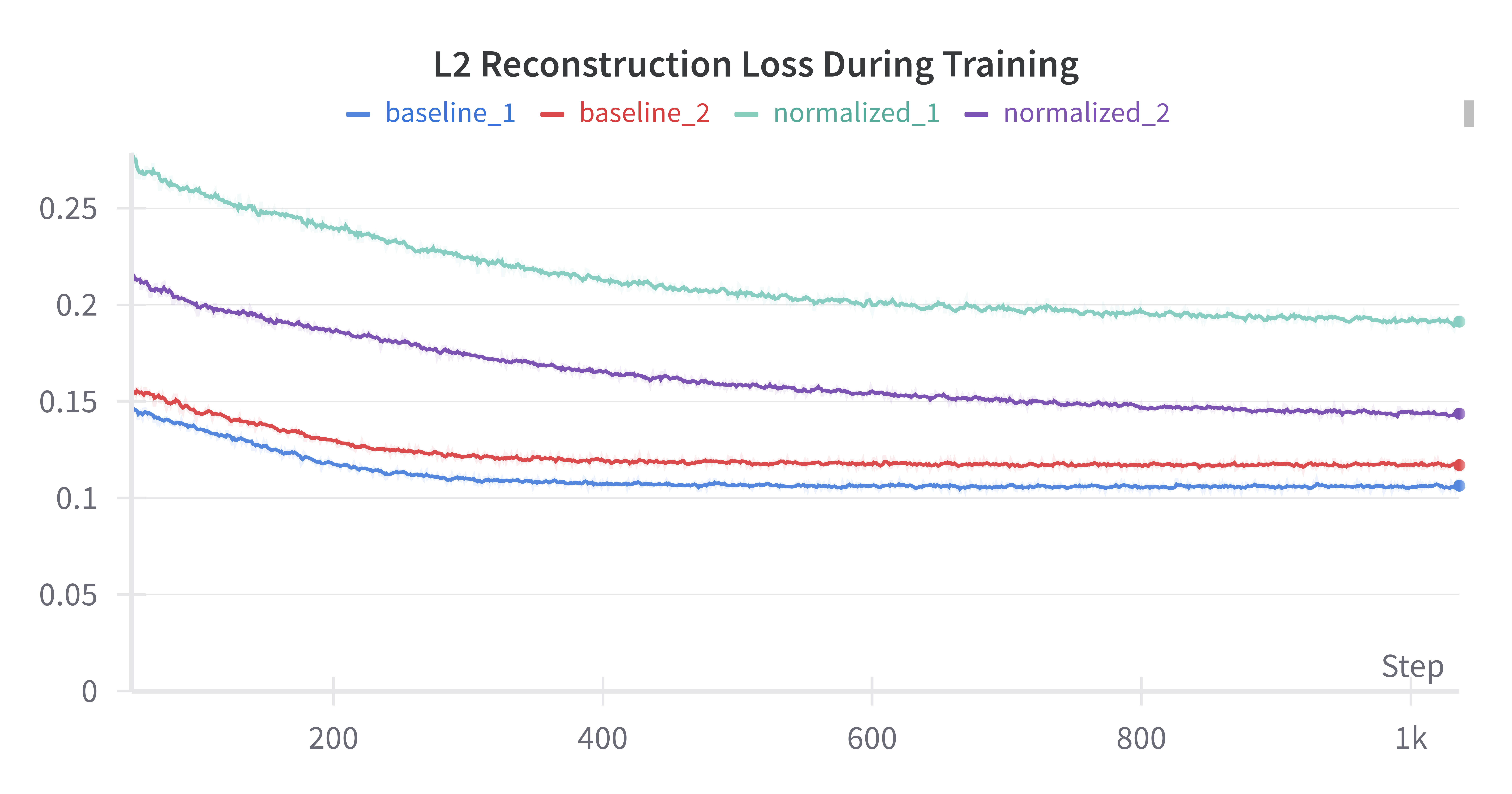
I suspect the reason of this is because NSAE learns a non-unit norm dictionary, and this dictionary have to capture all the norm information with a fixed size, whereas the original SAE can learn directions and add norm information through the feature activations. 

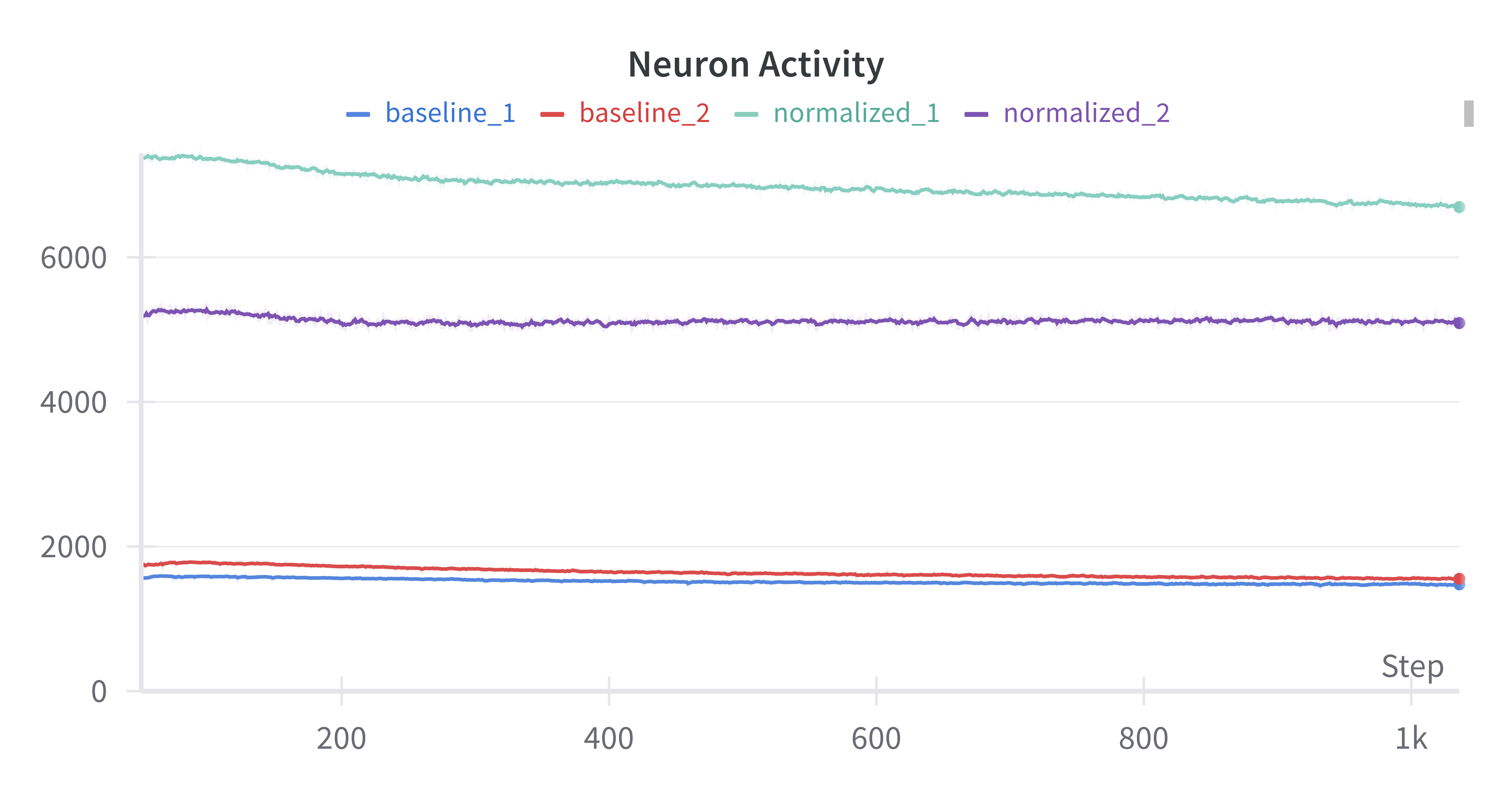
Another metric that I don't know how to interpret is the neural activity. In NSAE, the neural activity are significantly higher than the original SAE:

Lastly, the experiments conducted are relatively small in scale due to limitations in compute. Moreover, due to the change of the loss function, it's hard to directly match the scales of $L_0$ between the baseline and the experiment group. 

Future Work

I suggest future work to go along the following directions:

1. Investigate other factors that might caused the $L_0$ inconsistency across layers. I proposed a conjecture that it might be the difference in discreteness of source model input activations across layers that caused this inconsistency. 
2. Interpret the learned feature dictionary of NSAE. Future work can further investigate the feature vectors, especially the pillar vectors and direction vectors, and find interpretations for them. 

Appendix

Hyperparameters

I varied the hyperparameters l1_coefficients and the optimizer learning rate lr. For the two normalized groups, I also set the standard deviation of the Gaussian noise $\sigma$.

	baseline 1	baseline 2	normalized 1	normalized 2
l1_coefficient	0.001073	0.0009642	0.00004065	0.0000965
lr	0.0006275	0.00005584	0.0009045	0.000657
$\sigma$	N\A	N\A	1	1

Table A1. Hyperparameters used for training that varied for different runs

expansion_factor	16
context_size	256
source_data_batch_size	16
train_batch_size	4096
max_activations	100,000,000
validation_frequency	5,000,000
max_store_size	100,000
resample_interval	200,000,000
n_activations_activity_collate	100,000,000
threshold_is_dead_portion_fires	1e-6
max_n_resamples	4
resample_dataset_size	100_000
cache_names	blocks.{layer}.hook_mlp_out

Table A2. Fixed hyperparameters for all runs

Related Work

Riggs et. al. [LW · GW] proposed to use Sparse Autoencoders (SAEs) to discover interpretable features in large language models. Later, Wright et. al. [LW · GW] identified the Feature Suppression effect in SAEs and argued that the $L_1$ loss induced smaller feature activations that harmed reconstruction performance. Wes Gurnee [LW · GW] observed that the reconstruction errors in SAEs are empirically pathological, and compared different norm-aware interventions to the source model's inference. Results show that replacing the original residual state with SAE significantly changed the model's predictions, especially in deeper layers. 

1. ^{^}

   In this and the following examples, I used the residual states from the MLP layer.

2. ^{^}

   This is a reasonable assumption, as data in Figure 13 (baseline) show that most feature vector pairs in the original sparse autoencoder have cosine similarities in the range of $(-0.2,0.2)$.

3. ^{^}

   Empirically, $||x^{\prime }|{|}_2\approx 0.9||x|{|}_2$, which is close enough for our analysis.

4. ^{^}

   For computational efficiency, I randomly sampled $1,000,000$ features from the cosine similarity matrix.

5. ^{^}

   $L_0$ collected from step=3000. Input norm sampled from a relatively small sample of random text. This text is the same as the text used to generate figure 3, 4a, and 4b.

18 comments

Comments sorted by top scores.