Singular Learning Theory for Dummies

post by Rahul Chand (rahul-chand) · 2024-10-15T21:13:55.842Z · LW · GW · 0 comments

Contents

  Background
    Broad Basins
  Starting with SLT
  Building onto SLT
    SLT and physics
  Fisher information and Singularities  
  Limitations
None
No comments

In this post, I will cover Jesse Hoogland's work on Singular Learning Theory. The post is mostly meant as a dummies guide, and therefore won't be adding anything meaningfully new to his work. As a helpful guide at each point I try to mark the math difficulty of each section, some of it is trivial (I), some of it can be with followed with enough effort (II) and some of it out of our(my) scope and we blindly believe them to be true (III).

 

Background

Statistical learning theory is lying to you: "overparametrized" models actually aren't overparametrized, and generalization is not just a question of broad basins

Singular Learning Theory (SLT) tries to explain how neural networks generalize. One motivation for this is that the previous understanding of neural network generalization isn't quite correct. So what is the previous theory and why is it wrong?

Broad Basins

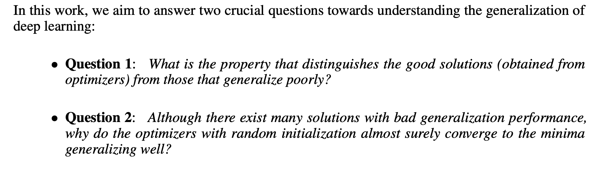
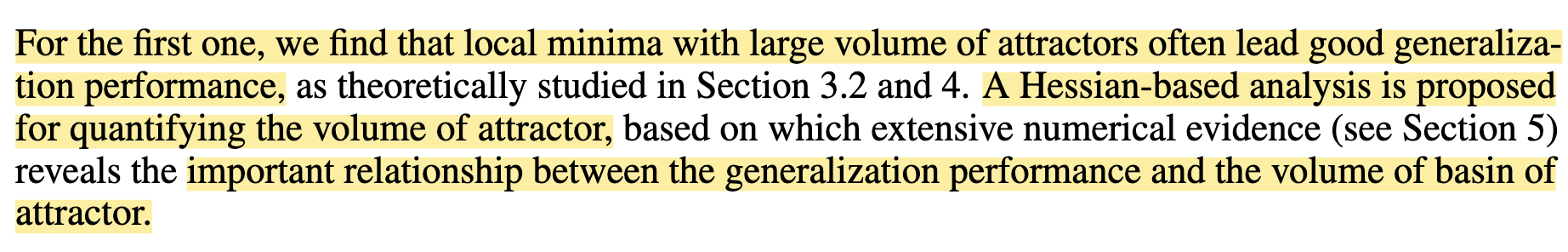
Below are excerpts from "Towards Understanding Generalization of Deep Learning: Perspective of Loss Landscapes"^[1] that summarize the logic behind broad basins theory of generalization

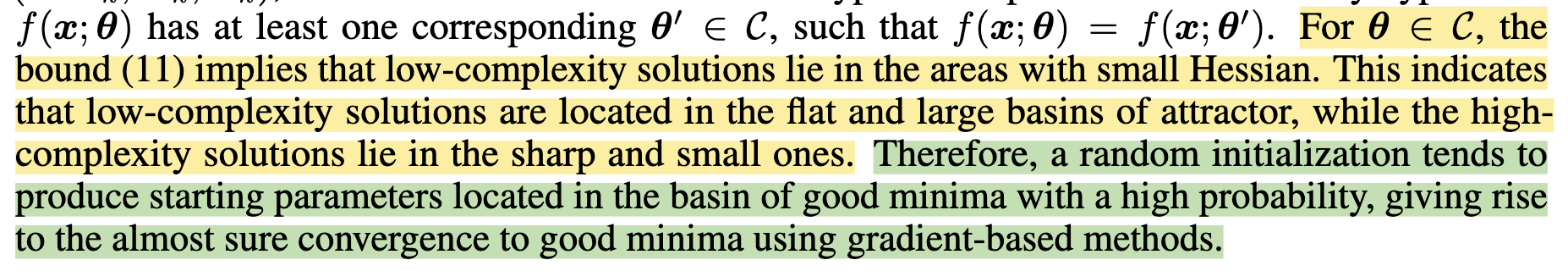
According to SLT there are two issues here. First, finding volume of a basin in the loss landscape by approximating it via hessian isn't accurate and second, the reason why models generalize has more to do with their symmetries than with with the fact that intialization drops the NNs in a good "broad basin" area.

Starting with SLT

A lot of basic maths for SLT is already covered in the original blog post. Here I will try to go over small questions that one might have (atleast i had) to get a clearer picture

What we know so far? (Math difficulty I)

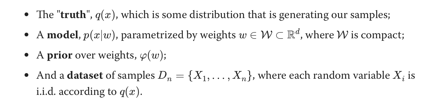
1. We define the truth, model and prior. The model is just the likelihood. These are standard bayesian terms.
2. Based on the above we know how to formalize the posterior & model evidence, p(w|D_n) & p(D_n) in terms of the likelihood and prior. Usually we stop at the posterior part, we are happy to get the p(w|D_n) for the model, but here we are interested in p(D_n) as well.

3. Why are we interested in $p\left(D_n\right)$ isn't our aim just to get the w that maximizes $p\left(w|D_n\right)$ ? 

   We are interested in $p\left(D_n\right)$ since it gives us the ability to not only tell what is the best w but the best architechure itself. So e.g. if you have some data D and you want the best w, and you are not sure what layer of neural network to chose, if we could magically make $p\left(D_n\right)$ tractable then we could get $p\left(D_n\right)$ for 10 layer neural network vs. 12 layer and find out which class of models better fits my data (and then get the $w_0$ later)

4. But whenever we are discussing bayesian, don't we always talk about how p(D_n) is intractable? Yes, we run it to the same problem here. We need two things to get us out. Both are Math level II. First, Laplace approximation^[2] where we can approximate the prior with a gaussian, and then how to use it to derive an approximation for model evidence^[3]

So after this, we end up with following model selection criterion

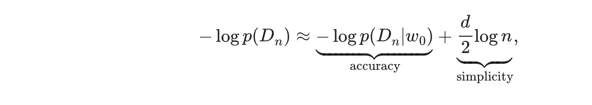
Which means that for a class of models we are interested in (W), the model evidence depends on how accurately your best w ($w_0$) increases the likelihood and how simple your model is (the value "d"). So you can either have a complex model which gives you great likelihood (lower training loss) but due to its $d$ being higher the model evidence will be lower and vice versa where you can have higher training loss but survive due to lower d^[4]

---

Building onto SLT

The idea behind SLT is that this Laplace approximation is not accurate for the models we care about^[5] (like NNs) and therefore the above formula also doesn't apply and therefore doesn't explain generalization. The class of models we care about are non-regular models A regular statistical model class is one which is identifiable (so $p(y|x,w_1)=p(y|x,w_2)$ implies that $w_1=w_2$). As we can see NNs are not regular since many different w's can correspond to same output. In the rest of the section, we discuss how we build up on the new approximation for model evidence that works for non-regular (singular models).  

SLT and physics

To start off we try to make an analogy between generalization in ML and thermodynamics. We will define bunch of new terms (which are rehashes of terms we have already seen but each has an analogy to thermodynamics). Math difficulty II

1. $L_n$ = negative log likelihood = -1*(the sum of log of likelihood)
2. Next we write the model evidence in terms of $L_n$. We call this $Z_n$ (partition function). Partition function in thermodynamics connects microscopic properties of a system to its macroscopic properties. Similar to how model evidence integrates/sums over all the different w's . Partition function in thermodynamics is defined as  $Z=\int e^{(-E/kT)}g\left(E\right)dE$ 
3. We then use the "Helmholtz free energy equation" from thermodynamics to define F_n (free energy) in terms of model evidence/partition function. Free energy is the value that all systems tend to minimize to reach their stable state. F_n = -log(Z_n). So here higher model evidence = more stable = lower free energy
4. Next we connect the Hamiltonian (Total energy) of a system with the partition function. If you differentiate Z and take log of it you get $nLn\left(w\right)-\beta log\phi \left(w\right)$
    

The analogy of free energy is easy to understand, its something we want to decreaese. As far as partition function and Hamiltonian are considered I like to think of them as, the Hamiltonian shows the energy landscape of the system, while the partition function samples this landscape to yield thermodynamic properties.

We next normalize these terms to make them easier to work with

1. For $L_n$ we are interested in finding its minima, we subtract $L_n$ with the theoretical possible minima (so that we can then use other math tools like finding zeros of polynomials to find out $L_n$). What is the least value of $L_n$ achievable? Each term in L_n is $-log\left(x_i|w\right)$ and the minimum we can achieve is true $log\left(x_i\right)$ which is $q\left(x_i\right)$. So $L=L_n-S$ (where S is just summation of $q\left(x_i\right)$) This is similar to KL-Div. But this doesn't look exactly like KL-Div, does it? Usually KL-Div looks like $\sum q\left(x\right)log\left(q\right(x\left)/p\right(x\left)\right)$. Here we don't have the q(x) term because this is more of like an empirical KL-Div. Which means implictly we sample x from the underlying q(x) to calculate it, therefore

$$K\left(w\right)=\left(1/n\right)\ast \sum _i^{N}log\left(q\right(x_i\left)/p\right(x_i|w\left)\right)$$

     2. We next normalize $Z_n$ into $Z_{n_0}$. Why do we divide by product of $q\left(X_i\right)$? Because in the original Z term we have integration over all w, $prior\ast e^{(-nB{L}_n(w\left)\right)}$. $L_n\left(w\right)$ is equal to sum over $log\left(p\right(x\left)\right)$, which when raised to e becomes product over $p\left(x\right)$, so we normalize with product over $q\left(x\right)$. This finally gives us

Most of the motivation for this section is to compare it with how we see phase changes in thermodynamics and how small critical points affect the larger macroscopic system. If we just followed the maths we could have done it without introducing free energy etc. as well.

"The more important aim of this conversion is that now the minima of the term in the exponent, $K\left(w\right)$, are equal to 0. If we manage to find a way to express $K\left(w\right)$ as a polynomial, this lets us to pull in the powerful machinery of algebraic geometry, which studies the zeros of polynomials. We've turned our problem of probability theory and statistics into a problem of algebra and geometry"

---

Fisher information and Singularities  

So far we have not covered what we mean by singularities. In the broad basin explanation, the effective dimensionality or generalization was based on the hessian of the loss landscape basin we found ourselves in. For singularity theory it is the RLCT (Real Log Canonical Threshold) of the singularities (we will see definition below) that determine the effective dimensionality. 

What is RLCT? What does it measure and how do we arrive at it? 

In the above section, we derived K(w), the term we want to minimize (The minimum K(w) we can reach is 0 and we assume for the rest of the discussion that this is achievable in our case). So we are concerned with the following points. These w_0 are singularities. 

                                                    $W_0=\{w_0\mid K(w_0)=0\}$

Before arriving at RLCT we will cover a few more things

Fisher information ($I\left(w\right)$): This is measures how much information an observation carries about an unknown parameter. Higher fisher information means small changes in W lead to high changes in likelihood and vice-versa. Therefore our broad basins are areas where fisher information is small. 

Fisher information when evaluated at $w_0$ also is equal to the hessian (in regular models). This connects the point that we saw at the start (hessian = inverse volume of basin). So small hessian = small fisher information = high volume basin (broader basin)

 

The issue we run into is that for singular models the fisher information at $w_0$ becomes degenerate (excerpt from DSTL1 blog explaining this)

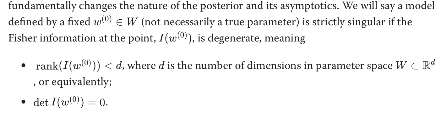
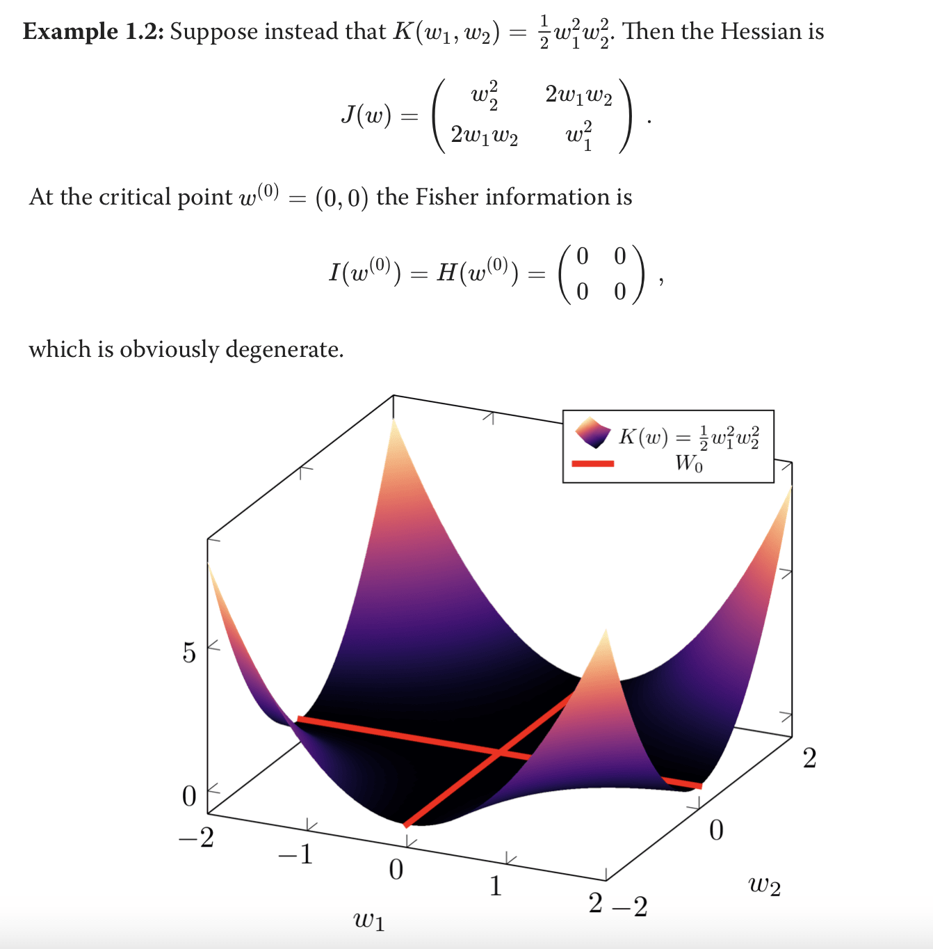
Fisher information at $w_0$ is degenerate for the models we are interested in (singular models). Which means using it as a measure of generalization (or more concretely, using it as a measure of effective diemnsionality) doesn't work. Following is an example from the DSLT1 blog which makes it easier to understand. Imagine you have this model where the loss function (K) is defined as $1/2w_1^2{w}_2^2$. The hessian/fisher at that point is all zeros which would first imply that we can't calculate the "volume" of this basin and second that the effective dimensionality is all zeros. But this is clearly not true,  there are more than zero "effective dimensions" in this model, a term that would intuitively imply $K\left(w\right)$ was identically zero, which it clearly is not. Thus, we need a different way of thinking about effective dimensionality. 

 

Now that we know for singular models, fisher information and hessian break down at points $w_0$. We look for another measure that can help us. In "Algebraic Geometry and Statistical Learning Theory" Watanabe derives the following

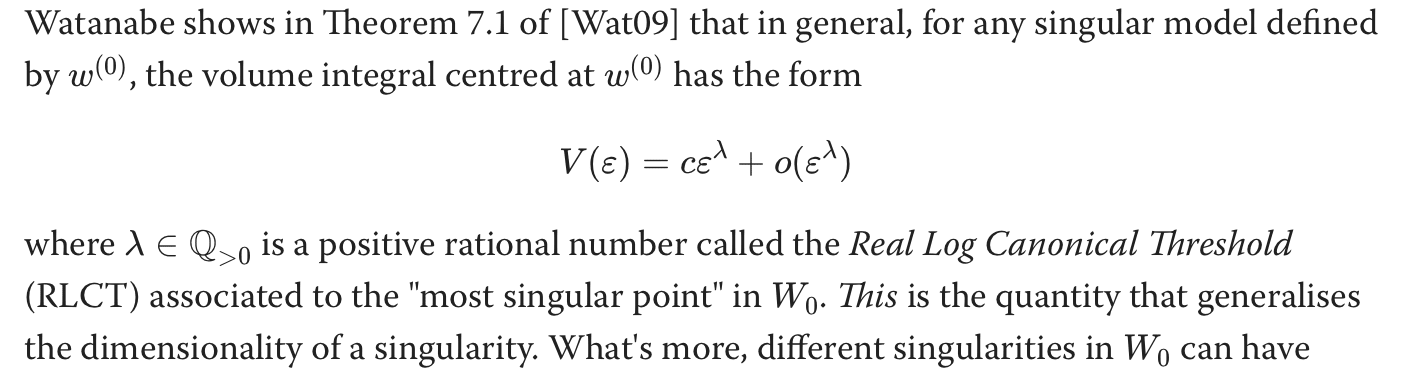
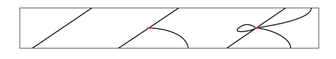
How do we arrive at this is much beyond mine and this blog's scope. But one thing we can keep in mind is that the RLCT is connected to how "bad" the singularity is. Like the diagram below the more "knots" there are, the worse the singularity is (more points where tangent is ill-defined). So RLCT($\lambda$) = a measure of effective dimensionality which can be used for non regular models = how complex the knots are = more complex the knots the more generalization. 

Another thing we see is that phase transitions during learning correspond to discrete changes in the geometry of the "local" (=restricted) loss landscape. The expected behavior for models in these sets is determined by the largest nearby singularities. We have covered what properties of loss landscape and $w_0$ result in better generalization. But we started off with two questions, 1) Finding what properties relate to generalization and secondly and more improtantly 2) Why do NNs generalize so well?

The whole going from BIC to RLCT covers the first question. Now what about the second? According to Hoogland, generality comes from a kind of internal model selection in which the model finds more complex singularities that use fewer effective parameters that favor simpler functions that generalize further.

"The trick behind why neural networks generalize so well is something like their ability to exploit symmetry". 

"The consequence is that even if our optimizers are not performing explicit Bayesian inference, these non-generic symmetries allow the optimizers to perform a kind of internal model selection." 

"There's a trade-off between lower effective dimensionality and higher accuracy that is subject to the same kinds of phase transitions as discussed in the previous section. The dynamics may not be exactly the same, but it is still the singularities and geometric invariants of the loss landscape that determine the dynamics."

That is, neural networks have so much capacity for symmetry^[6] that in most cases they end in loss landscapes with more complex singularities (therefore higher generalization). Remember in our previous explanation, we ended up at good regions with broad basins because the intitalization was much more probable to drop us there. Here, the structure of our models is such that during learning we tend to select complex singularties (which in turn leads to generalization)

This section has a bunch of maths that I skipped over. So it is possible to derive the degeneracy of the fisher matrix for non singular models by following the "Deriving the Bayesian Information Criterion only works for regular models" section (Math difficulty II). We then have two addition sections, first how to formalize volume in singular models (Volume of tubes) paper and then how we finally arrive at RLCT. I treat both of them as Math Difficulty III. 

---

Limitations

There are few limitations of the work, some of which Hoogland mentions at the end of the blog and some that he discusses in the comment section. I summarize them here, mostly qouting Hoogland himself

1) One subtle thing to keep in mind is that the above analysis is for bayesian inference and not for the SGD+NN kind of learning we are mostly interested in 

"Rather, it's making a claim about which features of the loss landscape end up having most influence on the training dynamics you see. This is exact for the case of Bayesian inference but still conjectural for real NNs"

2) RLCT is all good, but we cannot actually calculate them. Nothing in SLT tells us about how to evaluate if our w* are good or not. In some ways for now the hessian is a better indicator than RLCT (since its easier to calculate in general)

This is very much a work in progress. The basic takeaway is that singularities matter disproportionately, and if we're going to try to develop a theory of DNNs, they will likely form an important component. In any case, knowing of something's theoretical existence can often help us out on what may initially seem like unrelated turf

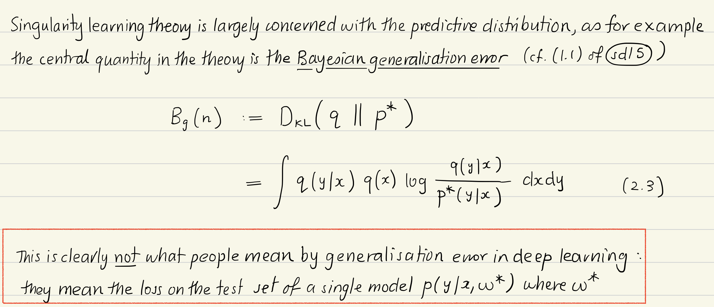
3) We don't really care about KL divergence though. We care about "generalization loss" which means your performance on the held out test dataset. How does this analysis extend?

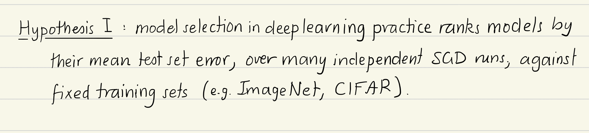
In the linked set of notes^[7] Hoogland makes an attempt to connect the test set loss and the model evidence (Bayesian generalization error) by connecting model selection with mean test error.  

There are some other limitations like the analysis being restricted to cases where n tends to infinity and the affect of regulairzation or other activation functions on the symmetry of neural networks. I felt that these were not as important as the ones mentioned above.

1. ^{^}

   https://arxiv.org/pdf/1706.10239

2. ^{^}

   Read more at https://en.wikipedia.org/wiki/Laplace%27s_approximation

3. ^{^}

   Derivation https://en.wikipedia.org/wiki/Bayesian_information_criterion#Derivation

4. ^{^}

   Wait but why are you using the model evidence as being same as generalization? Aren't they different? This is true and Hoogland covers this in additional notes which we briefly discuss at the end

5. ^{^}

   Explained in later sections, it has to do with fisher information becoming degenerate

6. ^{^}

   Lot of things contribute to this. First, matrix multiplication has permutation symmetry. There is symmetry due to skip layers. From attention mechanism etc. These are generic symmetries since all w belonging to this architecture have it. But with certain w, we can achieve even higher symmetries, certain parts of the model cancel out due to their weights or there output is 0 etc

7. ^{^}

   http://www.therisingsea.org/notes/metauni/slt6.pdf

0 comments

Comments sorted by top scores.