An evaluation of circuit evaluation metrics

post by Iván Arcuschin (arcus), Niels uit de Bos (nielius@gmail.com), Adrià Garriga-alonso (rhaps0dy) · 2024-04-15T19:38:53.457Z · LW · GW · 0 comments

Contents

  Summary
  Introduction
  Evaluation metrics
      Faithfulness
      Completeness
      Minimality
  Next steps
  Appendix
    Backup heads
      Remarks:
    Constant sub-circuit
      Remarks:
      Also, a minimal circuit can become non-minimal if you make the abstract model more granular
None
No comments

This work was produced as part of the ML Alignment & Theory Scholars Program - Winter 2023-24 Cohort, with mentorship from Adrià Garriga-Alonso. Equal contribution by Niels and Iván.

Summary

In this post we analyse the circuit evaluation metrics proposed by Wang et al. (IOI paper) and show that their specific formalisation allows for counter intuitive examples that don't always reflect the natural language properties they aim to capture. For example, some incomplete circuits can be made complete by removing components, and there exist faithful, complete and minimal circuits that have smaller circuits that are also faithful, complete and minimal.

Introduction

The main goal of Mechanistic Interpretability is to reverse engineer neural networks to make the learned weights into human-interpretable algorithms, hoping to develop a more principled understanding of deep learning. In this setup, models are seen as computational graphs, and circuits are subgraphs with distinct functionality. Circuits serve as a critical unit of measure to understand neural networks, since they allow us to analyse a model's behaviour only on a subset of its capabilities, usually by constraining the space of inputs to the ones associated with a specific task (e.g., the Indirect Object Identification task, as described by Wang et al.). Although circuits can be labelled, by assigning a human interpretation to some of its parts, in this post we focus on unlabelled ones.

In recent years, several techniques have been proposed for finding circuits (either manually or automatically). That is, given a specific task for which the model has a good performance, find the circuit (subgraph in the model) that is responsible for it.

Evaluation metrics

As part of the circuit discovery techniques, researchers have also designed and proposed circuit evaluation metrics that measure whether a circuit is "good" or not. However, although the natural language interpretation of these metrics usually seems reasonable, their specific formalisation can sometimes lead to counter intuitive results as we will show. In the following sections, we describe and present limitations for the three metrics proposed by Wang et al.: faithfulness, completeness, and minimality. Further details and specific examples can be found in the Appendix.

Notation: $M$ is the full model, $C$ denotes a circuit, and $F$ is a metric for measuring the performance of a circuit on the task (e.g. accuracy, or in the case of IOI, average logit difference).

Faithfulness

Natural language definition: "the circuit can perform the task as well as the whole model" (Wang et al., p.2)

Wang et al. formalise this metric as the fact that $|F\left(C\right)-F\left(M\right)|$ should be small (for some definition of small). In other words, if a circuit is faithful, then it can perform the task as well as the whole model.

It is important to note that measuring the score of a circuit (e.g., F(C)) involves removing all the components that don't take part in it (e.g., M \ C). This is usually done by ablation; this can be zero-ablation (replacing the activations in M \ C with zeros), resampling ablations (replacing with activations on randomly chosen corrupted data points), or mean ablations (replacing with the mean of the activations over some dataset) In any case, the specific choice of ablation might impact the final performance score for C. For example, if a sub-circuit is constant and non-zero on the dataset for the task, then zero-ablating that constant sub-circuit is likely to give a very bad faithfulness score, whereas resample-ablating will give a very good faithfulness score. While this is interesting, comparing different ablation methods is not the main focus of this post, and in our toy examples we assume zero-ablation for simplicity.

Completeness

Natural language definition: "the circuit contains all the nodes used to perform the task" (Wang et al., p.2)

Wang et al. formalise this metric as the fact that $\forall K\subset C$, the “incompleteness score”, $|F(C\setminus K)-F(M\setminus K)|$ should be small. In other words, C and M should not only be similar, but also remain similar under knockouts. They also propose 3 sampling methods for choosing which Ks to analyse, since doing it for all of them is computationally very expensive:  pick random subsets; use categories of circuit heads such as Name Mover Heads; greedily optimise K node-by-node to maximise the incompleteness score.

However, there are several limitations with this formalisation:

• This definition only looks at what happens when one removes parts of the circuit, instead of looking at what happens when one adds components. 
  • This means that this metric is not able to detect whether we can improve the circuit by adding components. Intuitively, one might think that would be the main purpose of a completeness metric.
• The completeness metric includes the faithfulness metric as a special case. If one takes K = emptyset, one gets exactly the faithfulness score, which means that a circuit needs to be faithful in order to be complete.
  • This is a problem in itself: ideally, the evaluation metrics would be orthogonal, but in this case, one of the metrics completely subsumes another. Consequently, if a circuit has a bad faithfulness score, it will also have a bad completeness score, and the completeness score does not give any indication about how you would improve the faithfulness or completeness score. 
  • As a result, overcomplete circuits, i.e., having extra nodes that are not relevant for the task, might have a big incompleteness score if those nodes hurt the circuit's performance. Even stranger, overcomplete circuits can be made complete by removing the extra nodes. For an example, see the constant sub-circuit in the Appendix (the circuit {A, +1}) is not complete according to this metric, while the smaller circuit {A} is complete). This same example works in the more realistic case where the subcircuit is not perfectly constant.

Minimality

Natural language definition: "the circuit doesn’t contain nodes irrelevant to the task" (Wang et al., p.2)

Wang et al. formalise this metric as the fact that $\forall v\in C,\exists K\subset C\setminus \left\{v\right\}\text{such that}|F(C\setminus (K\cup \left\{v\right\})-F(C\setminus K)|$ should be high. This is called the "minimality score".

The main limitation of this formalisation is that it works on a node level, but sometimes one is able to remove entire groups of nodes, making the circuit smaller and at the same time retaining performance on the task. See the example of a constant subcircuit in the appendix: {A, -1, +1} is minimal, faithful, and complete, but so is {A}. If the constant subcircuit in the example is not perfectly constant, but instead outputs some noise that hurts performance a little, we are still in a counterintuitive situation: {A, -1, +1} would still be minimal and complete, but there exists a smaller circuit {A} that is minimal, complete and more faithful. 

Another undesirable consequence of this definition is that it behaves incorrectly when you increase the granularity of your abstract model, e.g. if you split up a node in your abstract model into several nodes, or if you start ablating edges rather than only nodes. In particular, a non-minimal circuit can become minimal when you increase the granularity! You might expect minimal circuits to become non-minimal when you increase the granularity (because that means you can remove more granular components that don’t really matter), but you certainly wouldn't want the reverse to be the case! An example of this case is included in the constant subcircuit in the appendix.

Next steps

As next steps, we plan to either propose new ways to formalise the existing metrics (faithfulness, completeness, minimality), or propose new complementary metrics for measuring how "good" a circuit is. We also plan to analyse how the different ablation types impact circuit discovery techniques.

Appendix

We present different toy examples showing the limitations mentioned above. Every example has a short description and a table that lists for each subcircuit its completeness, minimality and faithfulness. The values in the column labelled F(C) are assumptions that are part of the setup for the example; the completeness, minimality and faithfulness are calculated based on those values.

Backup heads

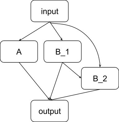
In this scenario, the output task relies on two sub-tasks: tasks A and B. Task A is performed by the node marked A, and task B can be performed either by node B_1 or by node B_2. Normally, however, node B_1 inhibits node B_2. When we ablate B_1, the node B_2 takes over. Backup heads occur naturally in transformers; see for example the IOI paper.

The following table shows the score for the circuit evaluation metrics when applied to different circuits in this example:

Circuit C	F(C)	Complete?	Minimal?	Faithful?
A, B_1, B_2	1 = F(M)	Yes	Yes: for every node in C we can choose a knockout circuit that shows a  performance change. For A, K = emptyset, for B_1, K = {B_2}, for B_2, K = {B_1}	Yes
A, B_1	1	No: knocking out B_1 damages the circuit, but not the full model	Yes	Yes
A, B_2	1	No: knocking out B_2 damages the circuit, but not the full model	Yes	Yes
B_1, B_2	0.5	No: not faithful	Yes	No
B_2	0.5	No: not faithful	Yes	No
B_1	0.5	No: not faithful	Yes	No
A	0.5	No: not faithful	Yes	No
ø	0	Yes	Yes	No

Remarks:

• This shows that to achieve a good score on the completeness metric, a circuit must contain all backup heads. That is a design decision that we think you can argue both for and against.
• In many of the cases, the completeness score adds nothing of value that was not already captured by faithfulness.
• Does this show anything else that’s interesting? If you use the relative sense of completeness, then it shows something interesting (circuits that are clearly not complete are listed as complete!), but otherwise not.

Constant sub-circuit

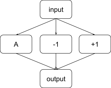
In this scenario, node A can perform the task perfectly by itself. However, the full model also contains another group of nodes that together are constant on the dataset for this task: the node labelled “-1” always outputs -1, and the node labelled “+1” always outputs +1 The output node in this diagram in turn sums the activation of nodes A, -1, and +1. As a result, if the outputs of the nodes -1 and +1 cancel out when both are included, but when precisely one of them is included, the summed output is completely wrong.

Again, the following table shows the score for the circuit evaluation metrics when applied to different circuits in this example:

Circuit C	F(C)	Complete?	Minimal?	Faithful?
A, -1, +1	1	Yes	Yes: if you remove any node, the new F-score is 0	Yes
A, -1	0	No: not faithful	Yes: if you remove -1, the score increases a lot, so -1 has high minimality score; for v = A, set K = {-1} to see that it also has a high minimality score	No
A, +1	0	No: not faithful	Yes (analogous to the above)	No
-1, +1	0	No: not faithful	No: whatever you knock out, the score stays 0	No
+1	0	No: not faithful	No: whatever you knock out, the score stays 0	No
-1	0	No: not faithful	No (analogous to the above)	No
A	1	Yes	Yes	Yes

Remarks:

• The full model is minimal, even though there is a constant sub-circuit consisting of the nodes -1 and +1 that can be removed and does not impact the performance on the task. In other words, the model without nodes +1, -1, is equally faithful and complete. This is a strong reason as to why the minimality score should be calculated for every subset, rather than for every single node.
• The circuit A, -1 is “minimal”, even though you can make it a lot better by removing the node -1.
• Although the circuit A, -1 is not complete, we can make it complete by removing the node -1, which is counter intuitive since incompleteness is usually interpreted as the "lack of something".

As was mentioned before, we can play with the circuit's granularity and we would obtain different results for the circuit evaluation metrics.

A non-minimal circuit can become minimal if you make the abstract model more granular.

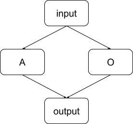
For example, if we group the nodes -1 and +1 together in a node labelled “O”, we get an abstract model that is less granular and looks like this:

Here, the full model is not a minimal circuit, because the node O does not have a high minimality score (since removing it does not change the performance as measured by $F$). In contrast, in the more granular model presented earlier, the full circuit is minimal. This shows that by making the model more granular, a circuit that was not minimal can suddenly become minimal.

 

Also, a minimal circuit can become non-minimal if you make the abstract model more granular

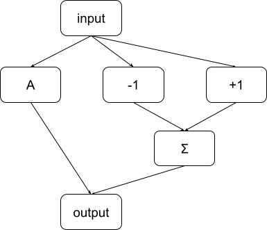
Another change we can make to the abstract model is the following: we introduce a node labelled “Σ” that sums the output of the nodes -1 and +1, after which that sum is added to the output of node A. This is the same computation as before: we’re only computing the sum A + (-1) + 1 in two steps, as A + ((-1) + 1).

This model is more granular than the first model: you can obtain the first model from this one by melting together the output node and Σ. However, in this case, the full circuit is minimal, because the node Σ does not have a high minimality score: removing it is basically equivalent to removing the entire constant subcircuit, so it does not impact the score as measured by $F$. This result is less surprising, though: you would expect that in more granular models, you can remove certain parts that are unnecessary for the task.

0 comments

Comments sorted by top scores.