Modelling and Understanding SGD

post by J Bostock (Jemist) · 2021-10-05T13:41:22.562Z · LW · GW · 0 comments

Contents

  SGD and Local Minima
  Monte Carlo
None
No comments

I began this as a way to get a better understanding of the feeling of SGD in generalized models. This doesn't go into detail as to what a loss function actually is, and doesn't even mention neural networks. The loss functions are likely to be totally unrealistic, and these methods may be well out-of-date. Nonetheless I thought this was interesting and worth sharing.

Imagine we have a one-parameter model, fitting to one datapoint. The parameter starts at $W=0$ and the loss is $L=-exp(-(W-2{)}^2)$. The gradient will then be $\frac{dL}{dW}=2(W-2)exp(-(W-2{)}^2)$.

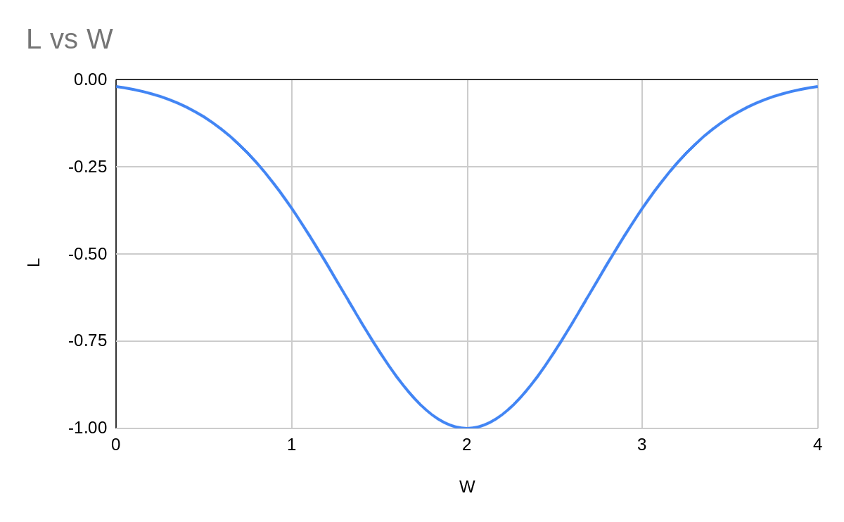
An imaginary continuous gradient descent will smoothly move to the bottom of the well and end up with $W=2$.

A stepwise gradient descent needs a hyperparameter $T$ telling it how much to move the parameters each step. Let's start with this at 1.

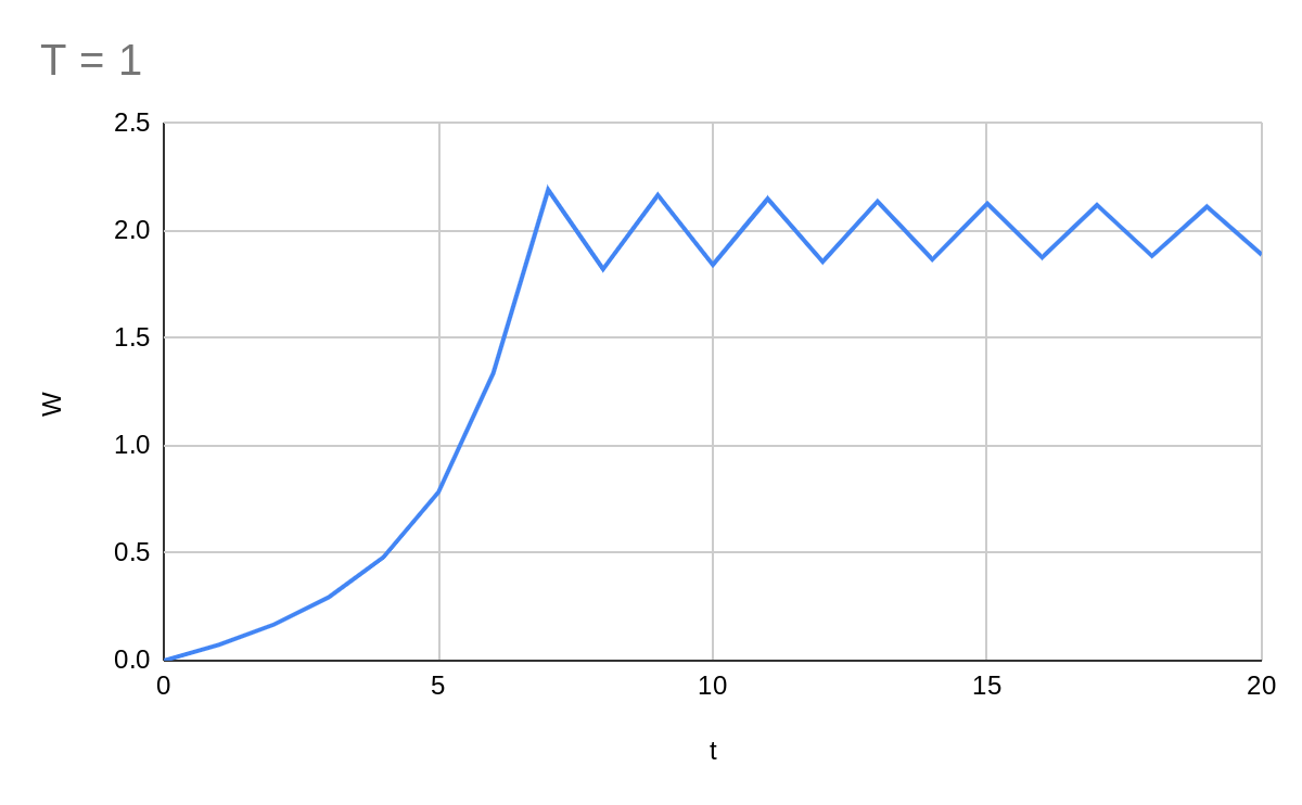
This gives us a zig-zag motion. The system is overshooting. Let's pick a smaller T value.

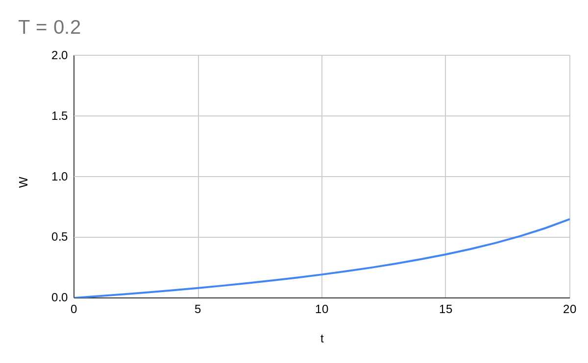
Hmm. Now our model converges quite slowly. What about 0.5?

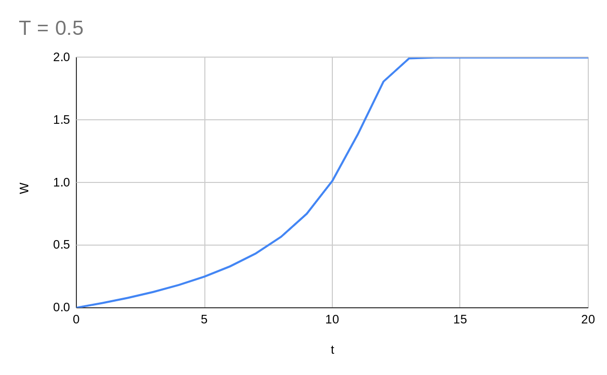
Much better. Seems that there's an optimal value of $T$, which we will later see depends on the spikiness of the loss function.

$T$ is not dimensionless and has the dimension of $W^2/L$, as $\Delta W=-T\frac{dL}{dW}$. Certain function-minimising methods like Newton's method use (for example) $\Delta W=-k\frac{dL}{dW}/\frac{d^{2}L}{d{W}^2}$ where $k$ is dimensionless. This is why different loss functions require different $T$ values.

SGD and Local Minima

What if we have two datapoints? Now $L=(l_0+l_1)/2$. Let $l_0=-exp(-(W-2{)}^2)$ as above but $l_1=-exp(-(W-2{)}^2)-exp(-100(W-1{)}^2)$. 

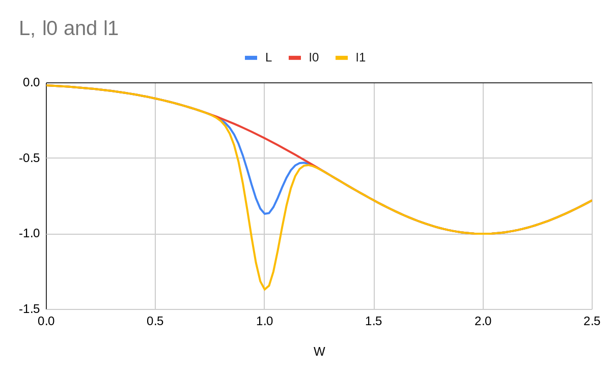
Now our loss function L has a new local minimum I think of this as "the pit". Where we end up depends on where we start. If we start at $W=4$ then we'll clearly end up at $W=2$ but if we start at $W=0$, then:

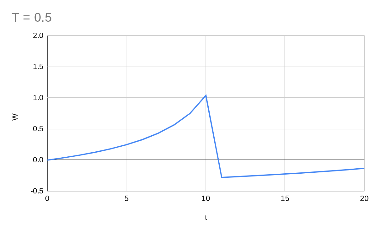
Huh, this isn't what I expected at all! The gradient must have been too high around the local minimum. Let's try with T = 0.05, which will be slower but ought to work better.

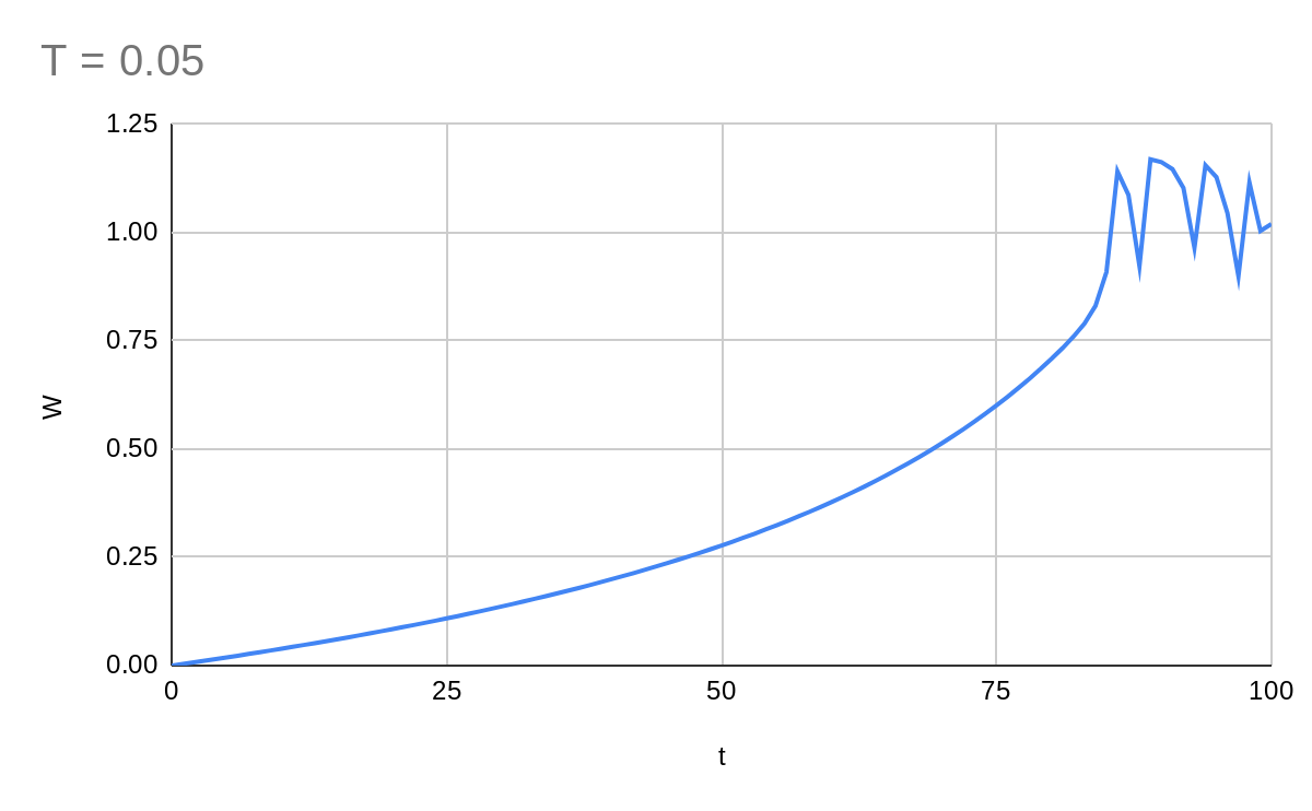
This is more like what I expected. Now our system is stuck in the local minimum.

But most modern gradient descent algorithms use stochastic gradient descent. We can model this here by randomly picking one of the two datapoints (with associated loss function) to descend by each step.

What happens now? Well now we have a chance to escape the pit. Let's say we're at the minimum of the pit. How many consecutive descent steps performed on $l_0$ will get us out of the pit?

Well by solving for the stationary points of $l_1$, we get $W=1.004$ and $W=1.196$. It turns out 5 steps of descent on $l_0$ will get us to $W=1.201$ which is out of the pit. Within 100 steps we have an 81% chance of getting out.

The interesting thing is that this doesn't depend much on the depth of the $W=1$ pit. If the local pit is twice as deep in $l_1$, then we only require one more consecutive step to escape it. If this is the case, then $W=1$ is in fact a global minimum in $L$. But because of SGD, it's not stable, and the only stable point is $p_0=2$! Clearly there is something other than overall minimum which affects how the parameter of the model changes over time.

What about smaller values of $T$? The number of consecutive steps in $l_0$ needed to escape the pit is inversely proportional to $T$. In the infinite limit as $T\to \infty$, we just converge on a continuous gradient descent, which will find the first minimum it comes to.

This reminds me of chemistry. It's as if the size of the step has to be big enough for the model to overcome some activation energy to cross the barrier from the $p_0=1$ pit to the $p_0=2$ one. This is the motivation for the letter $T$: temperature. The larger $T$ is, the more likely it is that the model will cross over out of the local minimum.

Monte Carlo

In fact we generally need significantly fewer than this. Starting around 1, one update on $l_0$ is enough to push us into the high-gradient region of $l_1$, which means even an update on $l_1$ will not move us back down into the centre, but rather to the left side of the pit, where a subsequent $l_1$ update might push us further towards the right.

Let's estimate the probability of escaping the pit in 100 steps as a function of T:

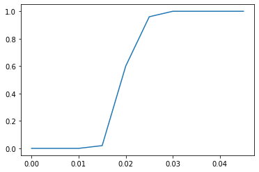
What about 1000?

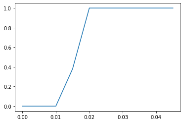
As we sort-of expected, it is easier to escape the pit than our original model predicted.

Let's look more closely at the region between 0.01 and 0.02:

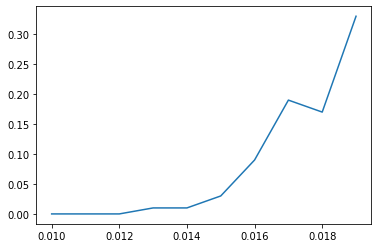
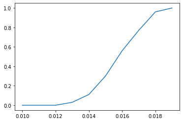
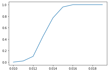
It looks roughly like the $log$ of the number of steps required to escape the pit is a function of T. Hopefully the later posts in this series will allow me to understand why.

0 comments

Comments sorted by top scores.