Visual demonstration of Optimizer's curse

post by Roman Malov · 2024-11-30T19:34:07.700Z · LW · GW · 0 comments

Contents

  Chapter 1: Optimization
  Chapter 2: Optimizator's curse
  Chapter 3: Bayesian remedy
  Chapter 4: Goodhart's curse
None
No comments

Epistemic status: I am currently taking this course, and after reading this post on Goodhart's curse, I wanted to create some visuals to better understand the described effect.

Chapter 1: Optimization

Veronica is a stock trader, and her job is to buy stocks, and then sell it at a specific time during the month. Her objective is to maximize profit. Here is the graph of how much money she will make if she sells at some specific time:

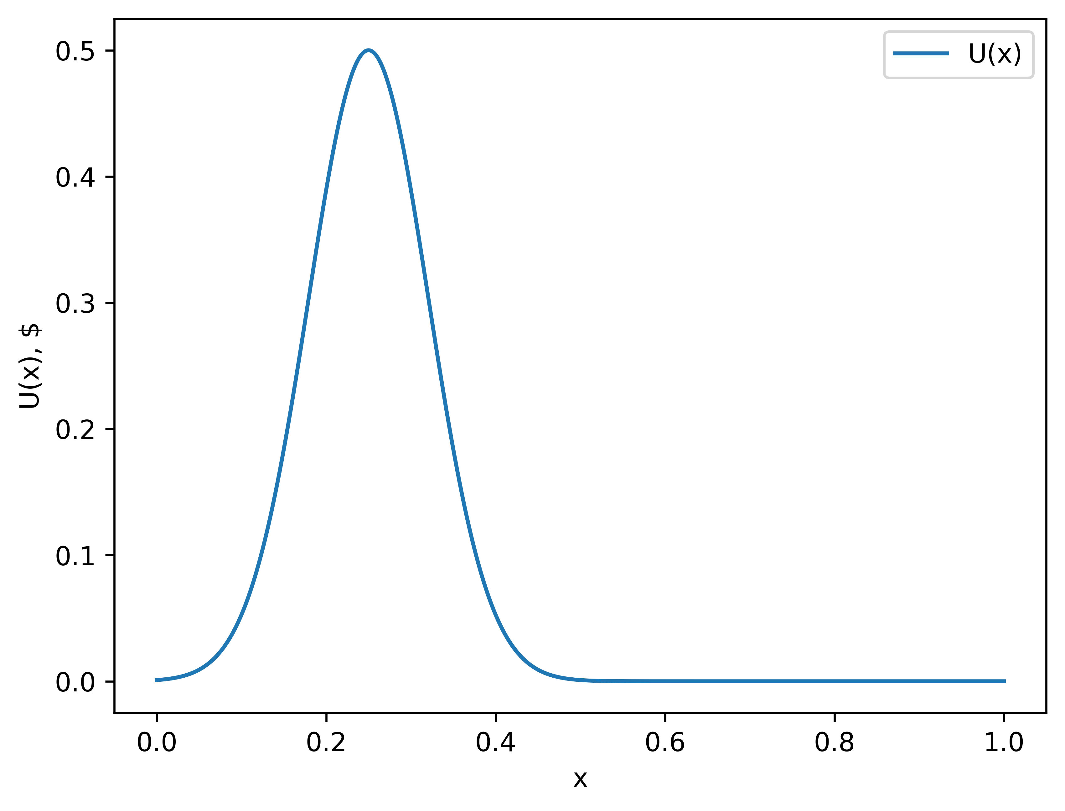
This can be called Veronica’s utility function $U\left(x\right)$, so if she sells at a time $x$, she makes $U\left(x\right)$ dollars.^[1]

But she does not have access to this function. She only has access to a giant supercomputer, which works like this: she presses the button, the computer chooses some random moment in the month $x$ and calculates $U\left(x\right)$. Running this computer takes a lot of time, so she can only observe a handful of points. After that, she can analyze this data to make a decision about the selling time.

Her current algorithm is as follows:

Algorithm 1

1. Run the computer $N$ times, generating $N$ pairs of the type $(x_i,U(x_i\left)\right)$.
2. Locate the maximum using argmax: $x_{max}=\underset{x_i\in \{x_1,\dots ,x_N\}}{\mathrm{argmax}}\left[U\right(x_i\left)\right]$
3. Sell stocks at the time $x_{max}$ and receive $U\left(x_{max}\right)$ dollars.

Here is the picture of how one such scenario might look like:

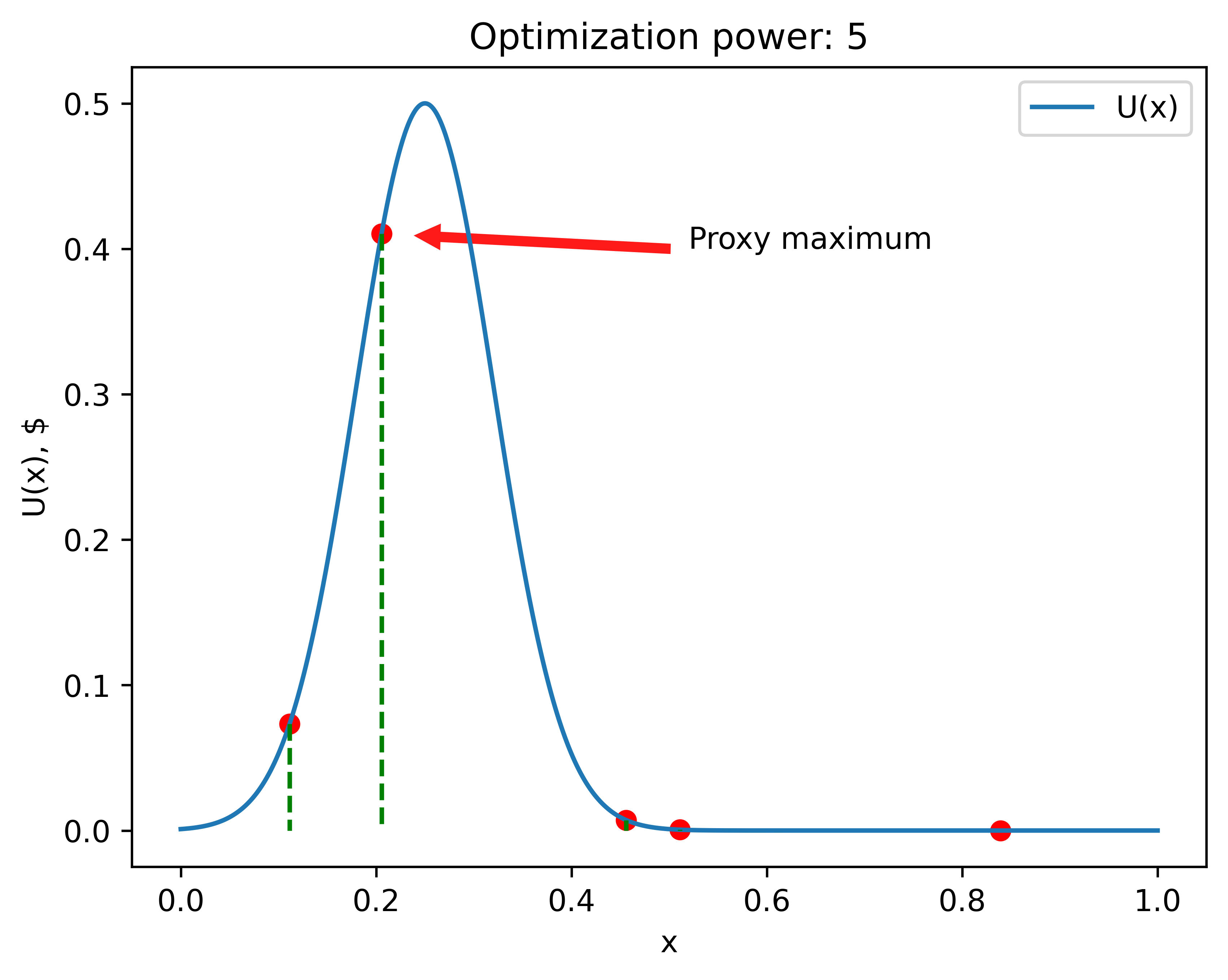
The number $N$ of observed points (aka the number of times Veronica pressed the button) will be referred to as 'optimization power'. The higher this number, the closer (on average) her proxy maxima will be to the actual maximum.

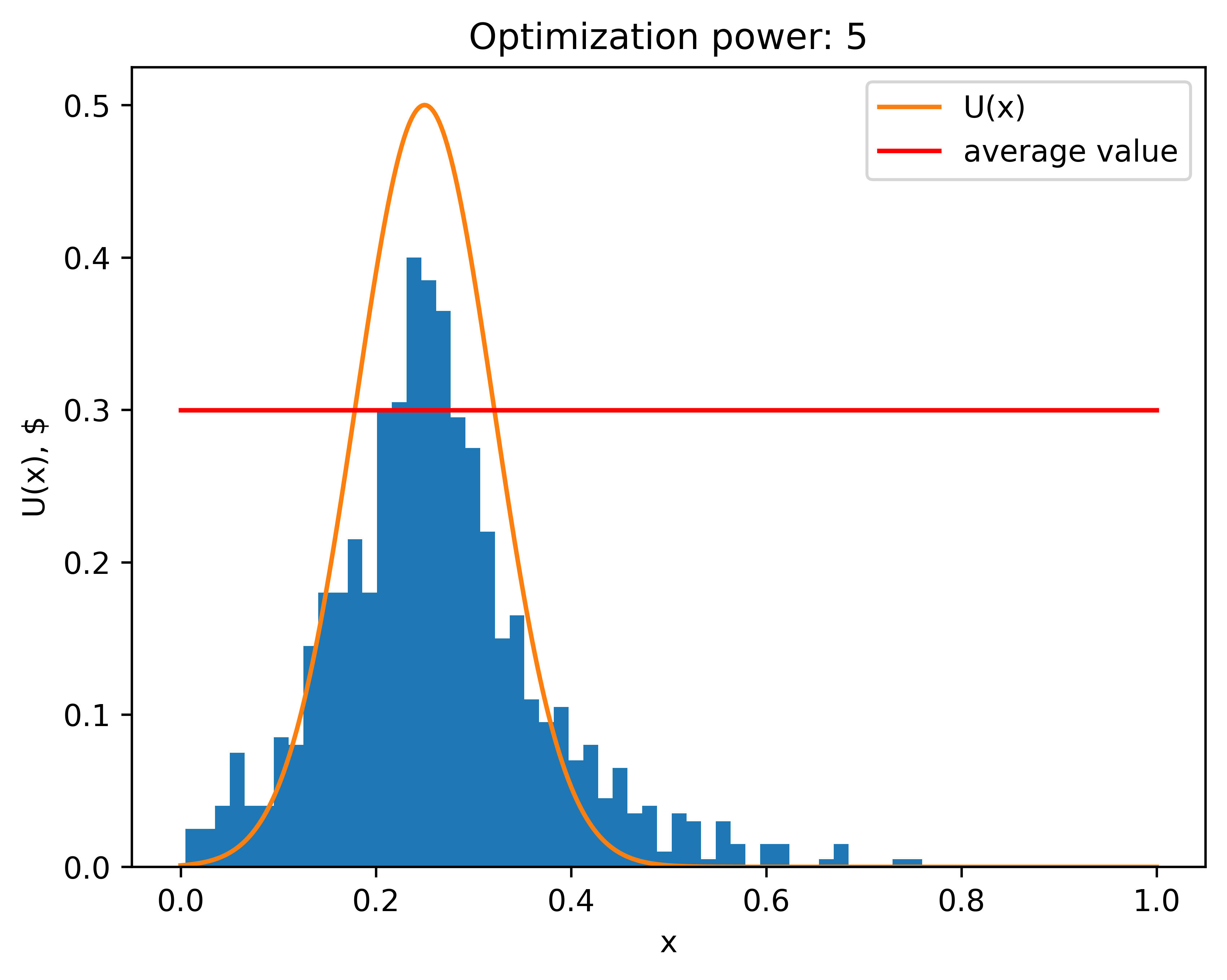
Here are 1,000 such experiments, in each of which the optimization power was 5. The bar chart is the probability density of the proxy maxima chosen by the Algorithm 1.^[2] We can see that points are clustering around the true maximum point ($x=0.25$). The “average value” is the average of the utility function $U$ Veronica obtains from those proxy maxima (the expected amount of money she makes with this algorithm). It is noticeably smaller than the actual maximum value she can achieve.

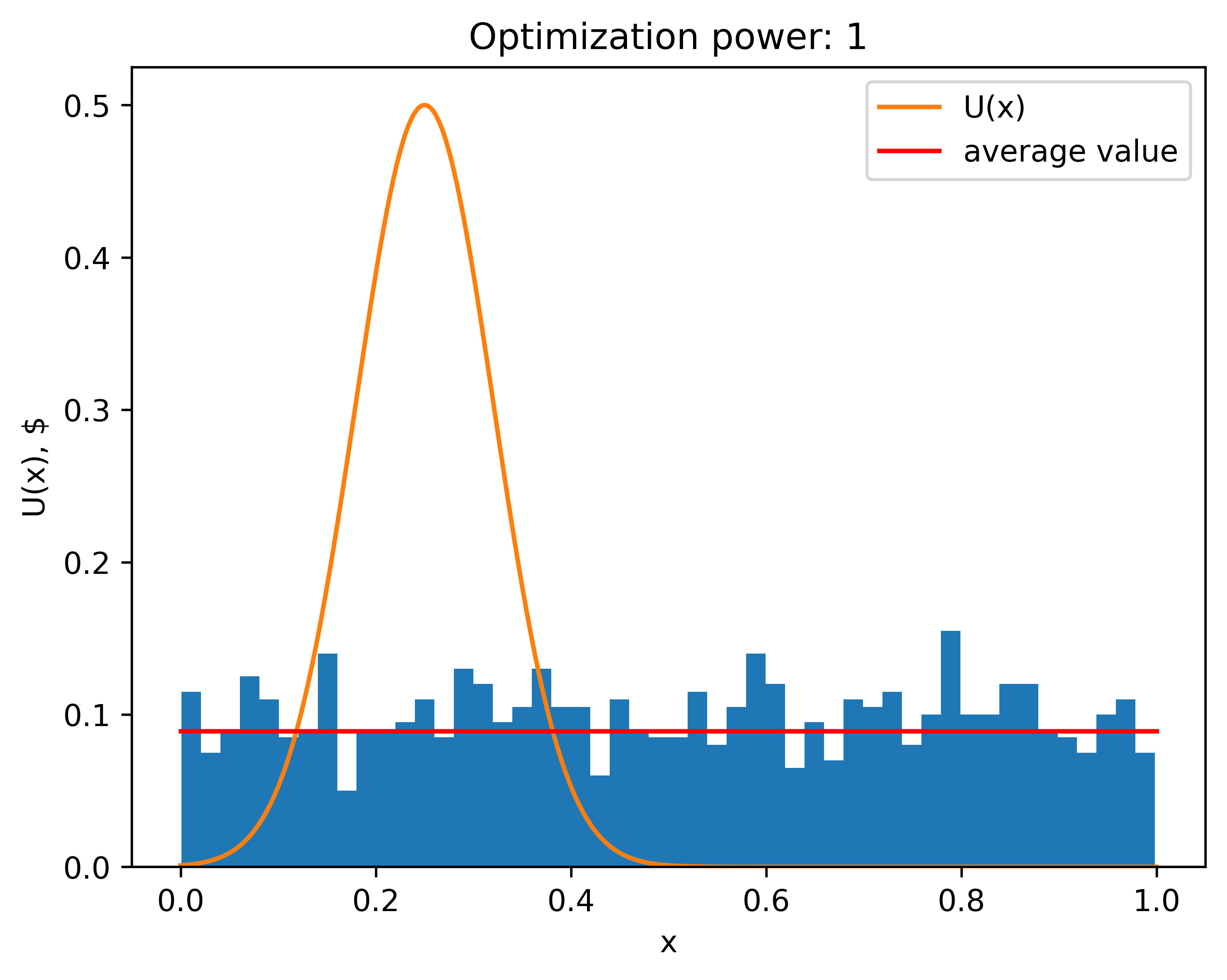
With the lowest optimization power ($N=1$) Veronica doesn't gain any information, and is her guess is equivalent to a random choice (since she is choosing from a single randomly selected point).

Here is what happens if she cranks up the optimization power (runs the forecasting supercomputer many times).

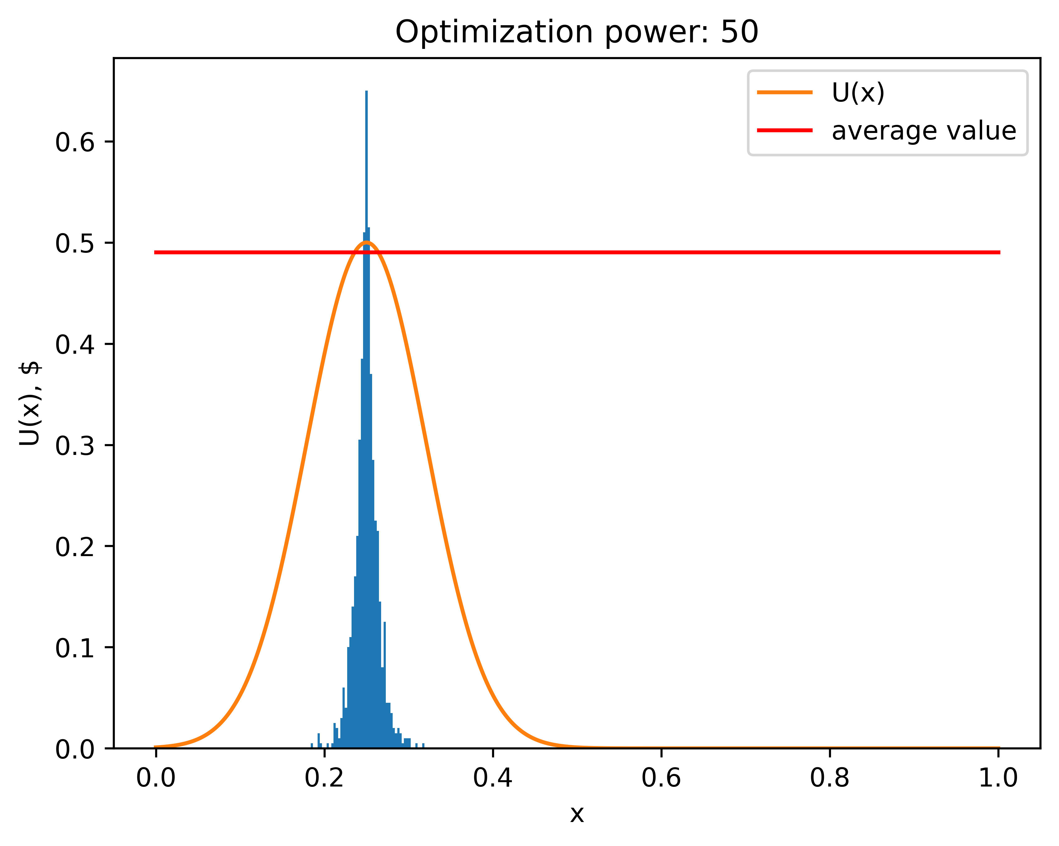
Her expected profit is now much closer to the actual maximum profit. Additionally, the distribution is much narrower: now proxy maxima are, on average much closer to the actual maximum.

Here is a graph of the dependence of the average value on the optimization power.

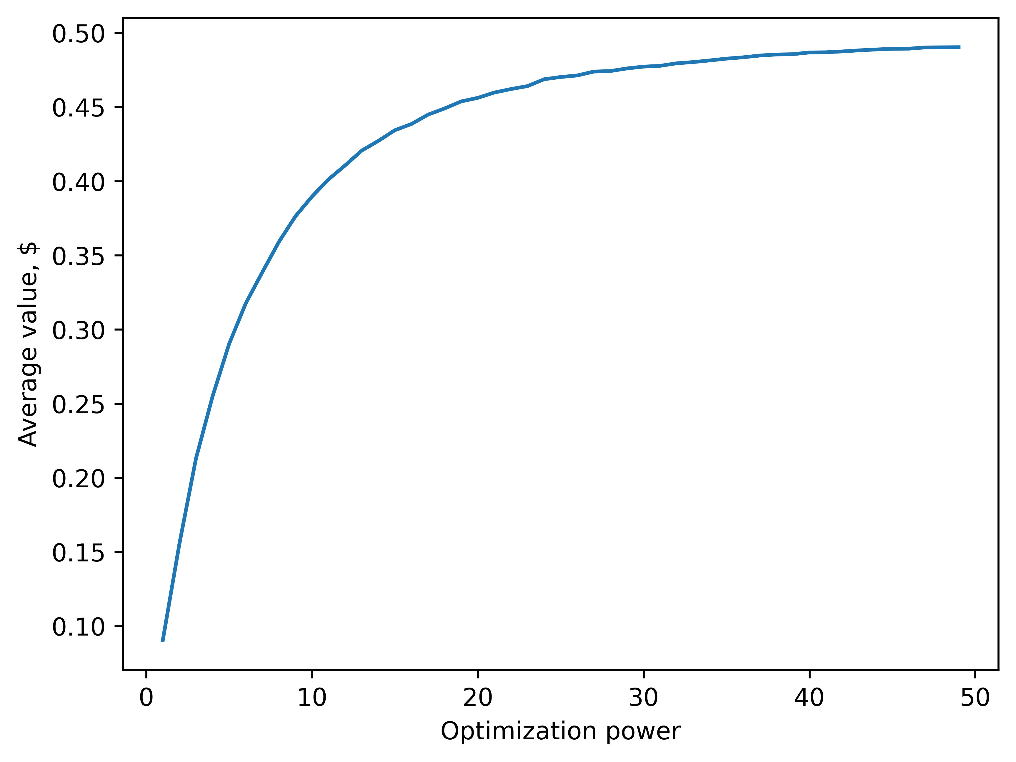
Notice how it increases monotonically (which shouldn't be surprising).

Chapter 2: Optimizator's curse

In reality, forecasting distant events is hard, and the further away the event, the harder it becomes. To account for that, we can add noise in Veronica's measurements of utility. In this example it would be the error in computed profits; and the further in time we try to make predictions, the harder it is, and that is reflected with purple area on the plot. In my model, what Veronica gets from the computer is the actual value of $U$ at that point $+$ gaussian noise. So now, the result of the computer's prediction is $(x_i,\tilde{U}(x_i\left)\right)$, where $\tilde{U}\left(x_i\right)$ is a noisy estimation of $U\left(x_i\right)$. Purple area represents $1\sigma$ interval, and $\sigma \left(x\right)=x^4$, so it increases with time. Notice that this is an unbiased estimation: on average, with a lot of samples, she would get closer and closer to the actual value of $U$.

Here's how one of these scenarios might play out.

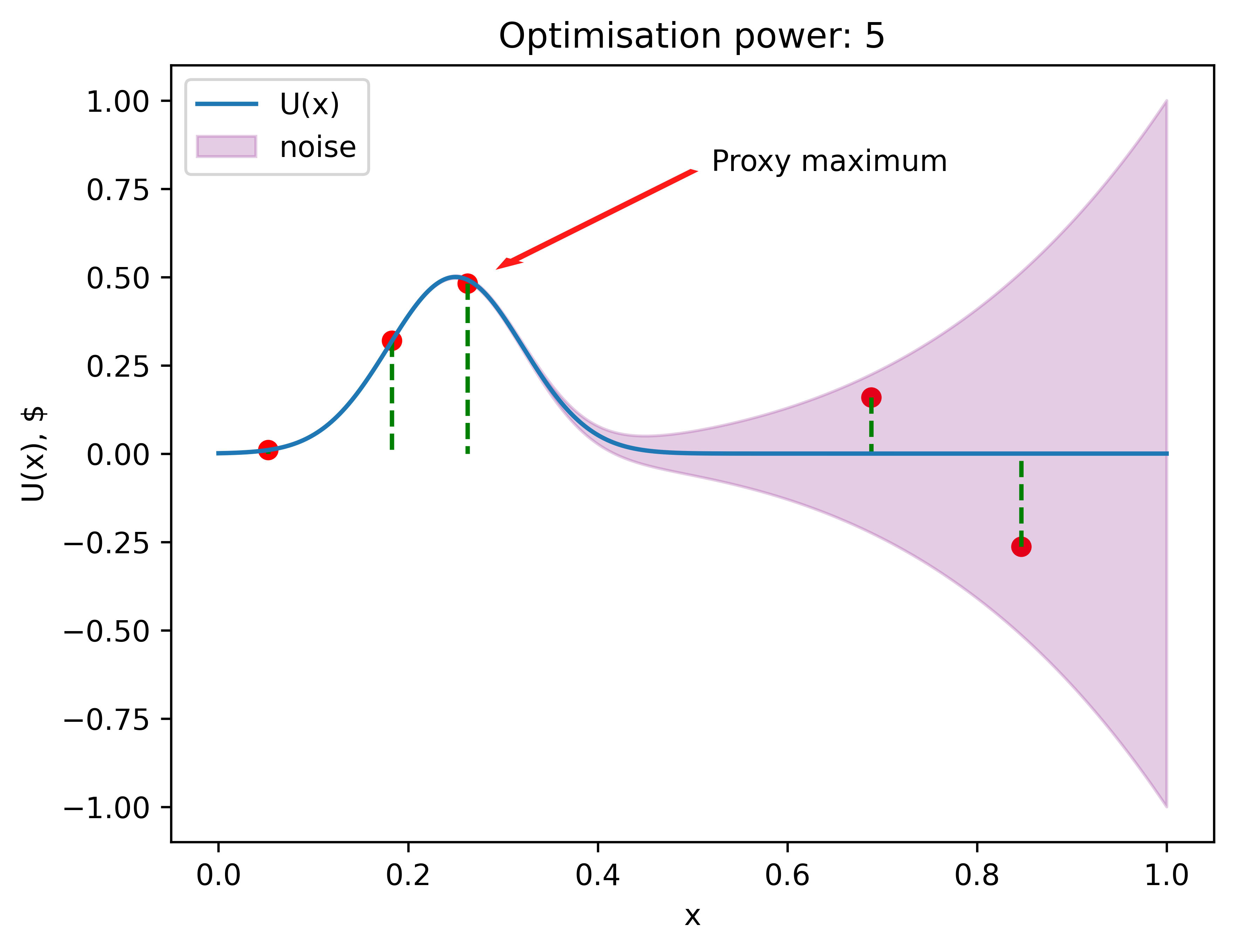
In this case, Veronica's proxy maximum lies near the actual maximum. However, that is not always the case.

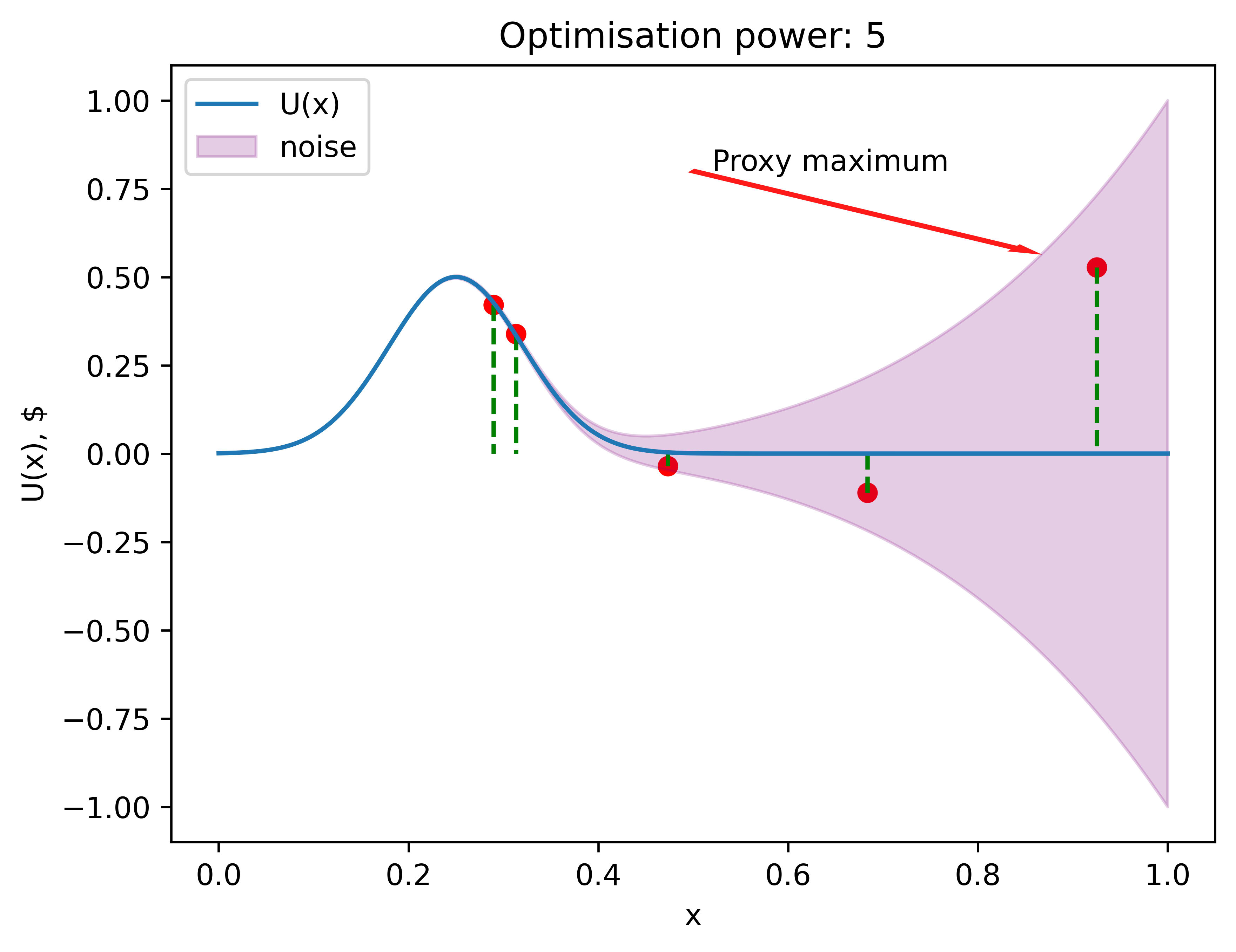
Sometimes, (as in example above) flukes from the noisy area are higher than the signal from the actual near-maximum area, and her chosen proxy maximum is way off.

Now let’s look at a distribution of proxy maxima (1,000 experiments).

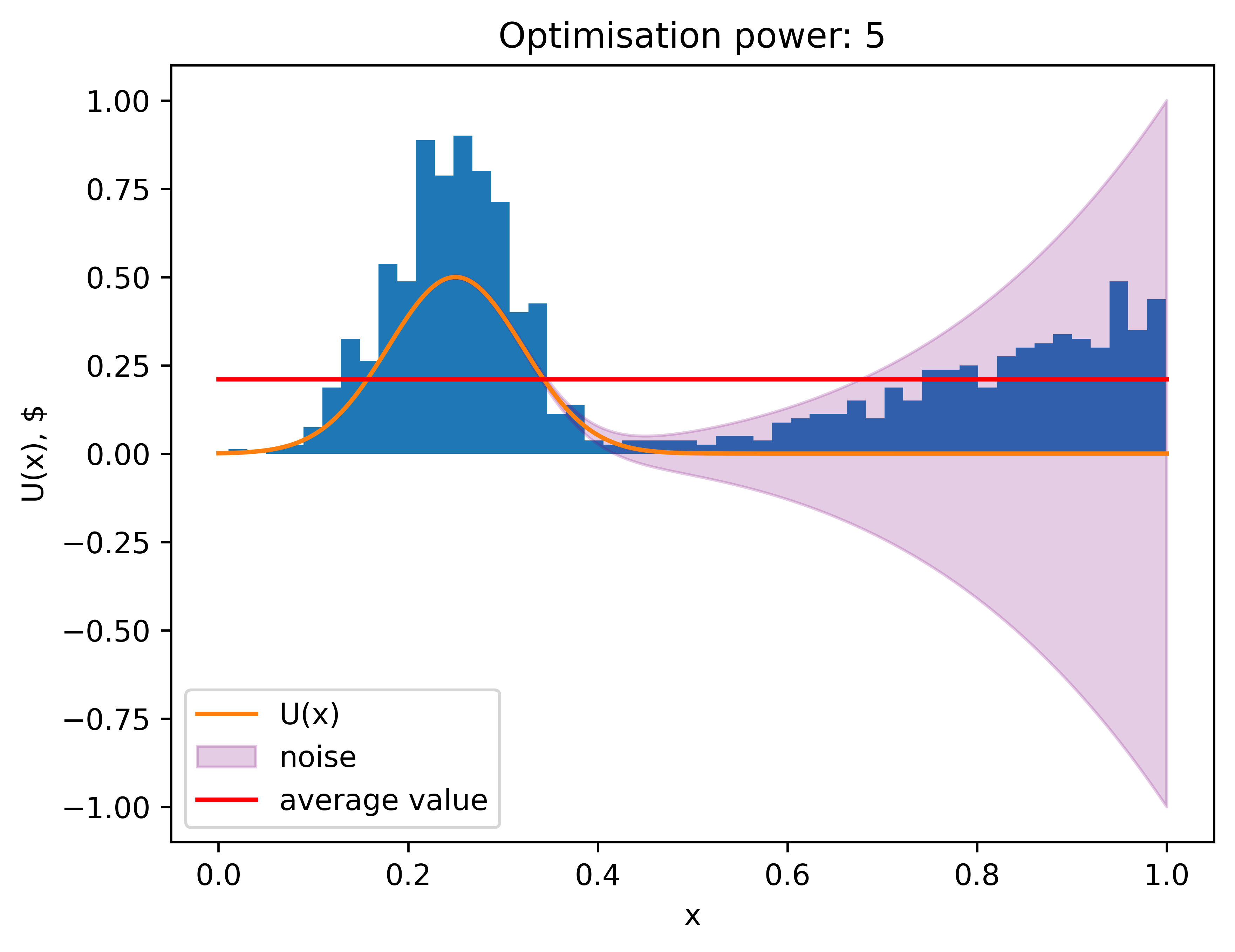
The average value decreased a bit, but that is to be expected, we introduced some obstacle. But notice how the distribution is bimodal: the noise we introduced caused some of Veronica's estimations of maximum to be completely off. That’s because when she samples, some of the points, which are located in the high-variance area have high noise-induced values, and this is not balanced with points with low noise-induced value, because those low points effectively do not “participate in the competition”. This effect is called Optimizer's curse: tendency of optimizers to seek high areas with high variance.

But surely, with the help of bigger optimization power Veronica can fix this, that helped her to make expected utility bigger before, right? But no! In fact (with the assumptions we made) it gets worse:

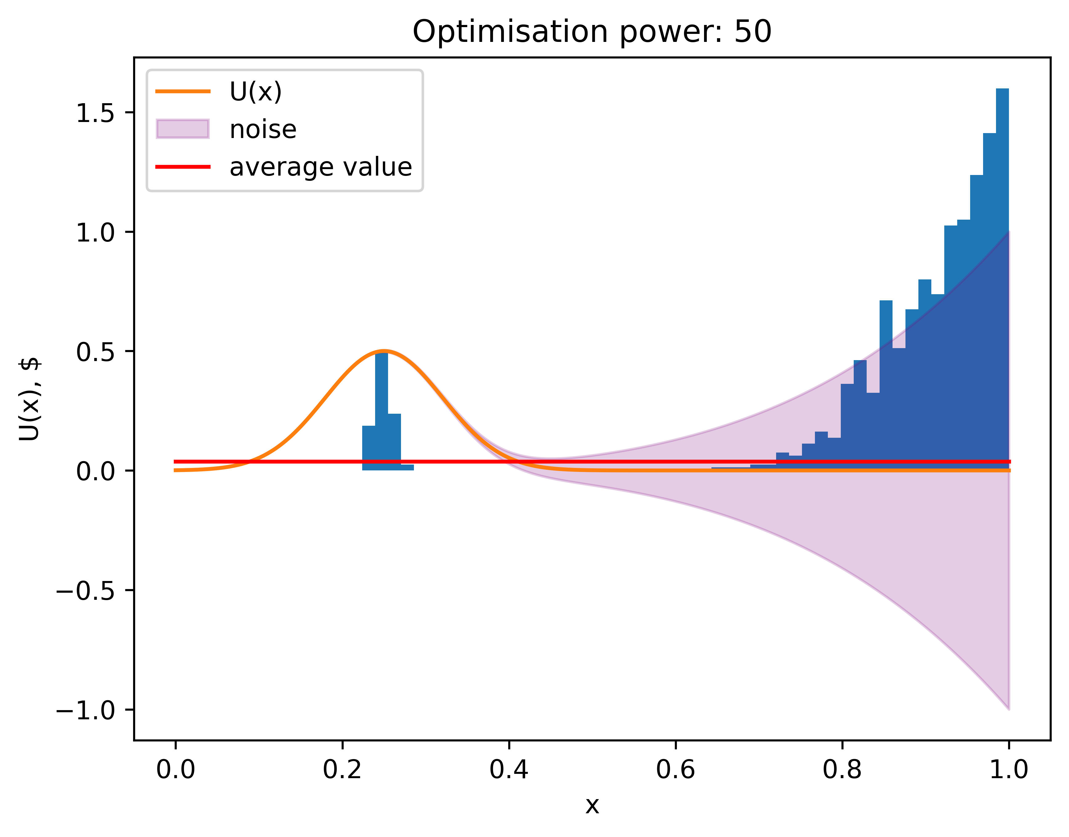
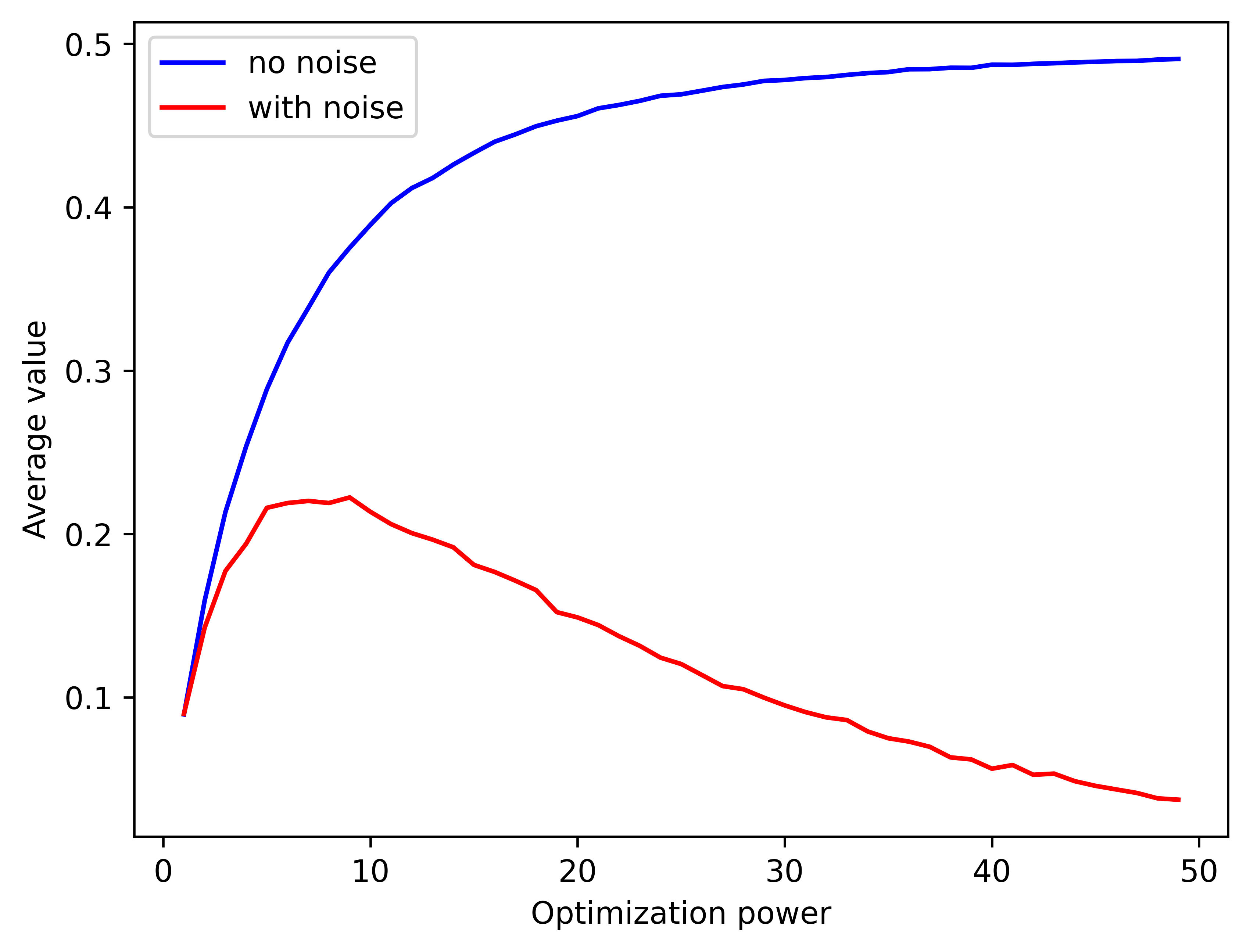
An increase in optimization power resulted in a lower average value because, with more samples, the probability that the highest point from a noisy area exceeds the actual maximum of the utility function increases. Here’s the graph of the average value with respect to optimization power. At some point, higher optimization power is worse than random sampling.

Chapter 3: Bayesian remedy

Now, before we see Veronica using Bayes theorem with her task, let's take a step back and look at an easy example of applying bayesian updates.

Roman is a physicist running an experiment. He observes the decay of some particle. He does not know the half-life period $t_{1/2}$ of this particle, and needs to infer it from observations.

Every time he sees a particle decay, he records how long it took. The probability density of this time is $\rho \left(t|t_{1/2}\right)=\frac{1}{t_{1/2}}\exp \left(\frac{t}{t_{1/2}}\right)$. This is called exponential distribution.

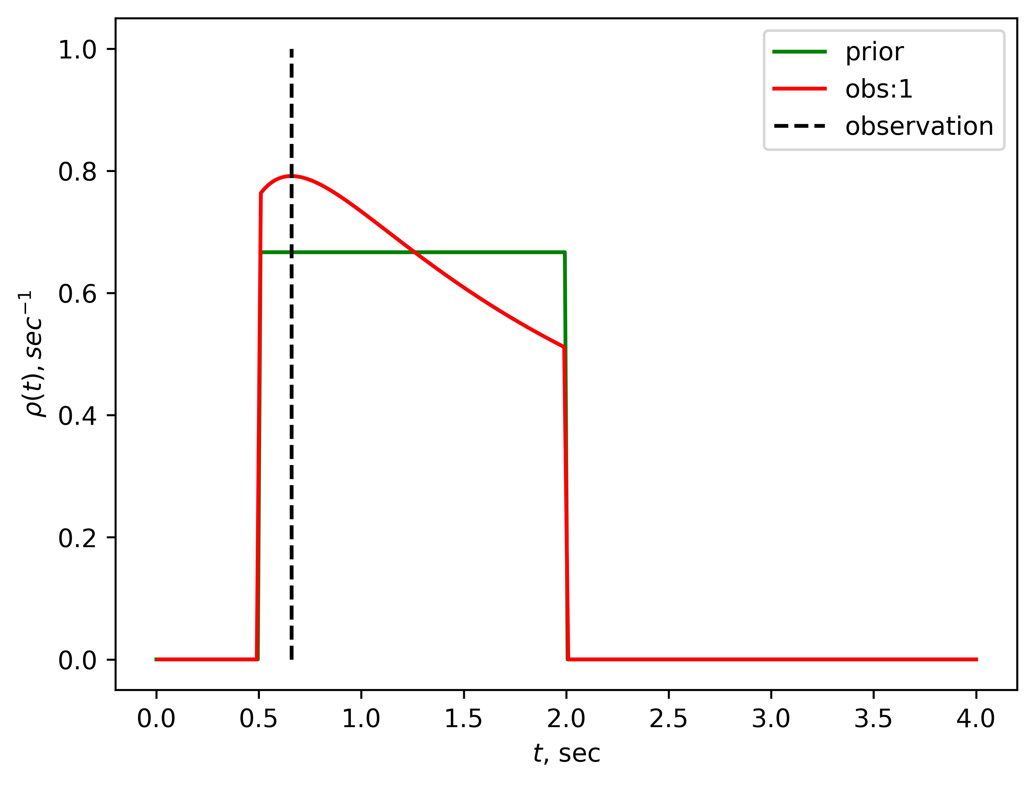
He knows that $t_{1/2}$ is somewhere between 0.5 and 2 seconds. His prior distribution on $\rho \left(t_{1/2}\right)$ might look something like this:

 

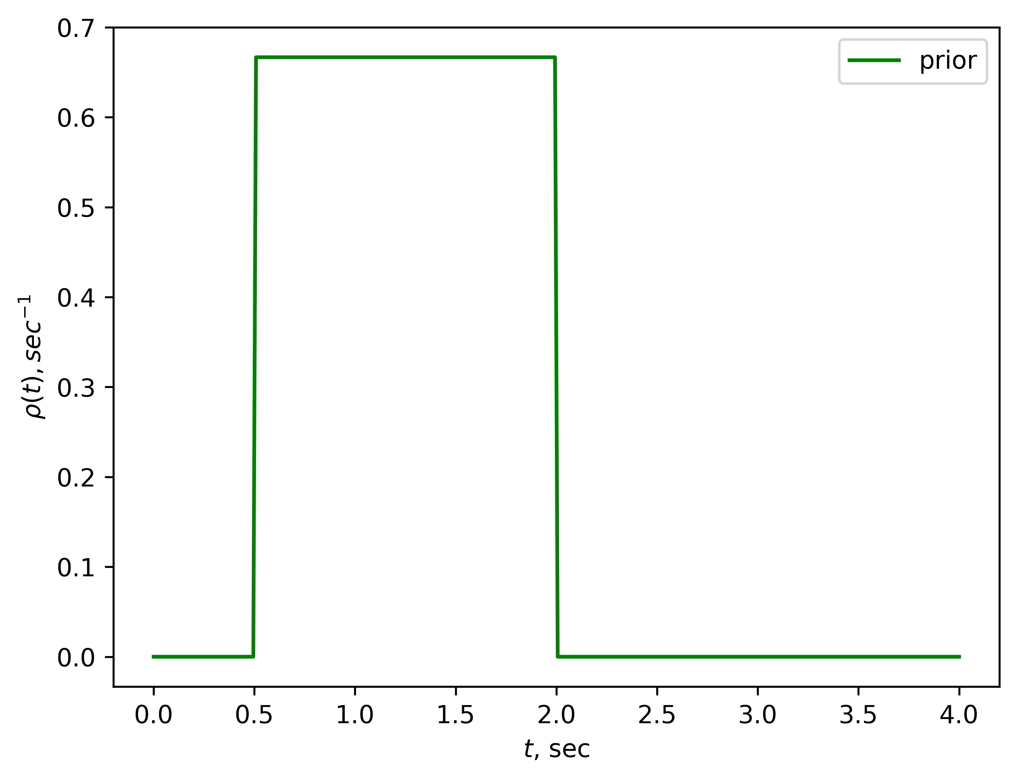
Each possible value of the $t_{1/2}$ is a hypothesis, and the prior distribution assigns some probability (in our case probability density) to each hypothesis. After Roman gets an observation $t_1$, he updates his beliefs about how likely each hypothesis is using Bayes's theorem:^[3]

$\rho \left(t_{1/2}|t_1\right)=\frac{\rho \left(t_{1/2}\right)\rho \left(t_1|t_{1/2}\right)}{P\left(t_1\right)}=\frac{1}{P\left(t_1\right)}\cdot \frac{2}{3}{1}_{[0.5;2]}\left(t_{1/2}\right)\cdot \frac{1}{t_{1/2}}\exp (-\frac{t_1}{t_{1/2}})$^[4]

The term in the denominator is a constant and can be calculated using normalization.

After the first observation, Roman's posterior distribution looks like this:

Then Roman can call the resulting distribution his new prior distribution (and he can do that because observations are uncorrelated) and keep doing the process. Here is a GIF of how that would look like:

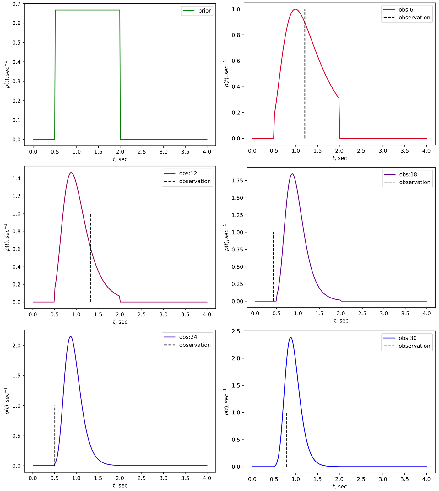
It gets narrower and higher,and in the limit, there should be a high peak around the true value of $t_{1/2}$ (in our case $t_{1/2}=1$ sec).

His algorithm is as follows:

Algorithm 2

1. Set some prior distribution  ${\rho }_0\left(t_{1/2}\right)$
2. Get the observation $t_i$ of a decay time of a specific particle.
3. Calculate posterior distribution using Bayes theorem: ${\rho }_i\left(t_{1/2}|t_i\right)=\frac{{\rho }_i\left(t_{1/2}\right)\rho \left(t_i|t_{1/2}\right)}{P\left(t_i\right)}$

4. Set this posterior distribution as the new prior distribution and return to step 2.

   ${\rho }_{i+1}\left(t_{1/2}\right)={\rho }_i\left(t_{1/2}|t_i\right)$

Now let's get back to Veronica and her stock trading problem.

To get the bayesian method working, Veronica needs a space of hypotheses. Each hypothesis is a distribution which generates observations, and with each observation she would narrow down this space of hypothesis. 

Before she runs a computer, she has some idea of what the utility function might look like. She thinks that it is a smooth function with a single peak, but she does not know the value of this peak or where it is on the $x$ axis. Also, she accounts for a potential noise in predictions from the computer.

Colormap of one such hypothesis (which shows with what probability each pair $(x,\tilde{U}(x\left)\right)$ can be outputed) with a specific value of peak hight $h=0.7$ and $x$-coordinate of this peak $\mu =0.3$ would look like this (the blacker the region, the higher the probability):

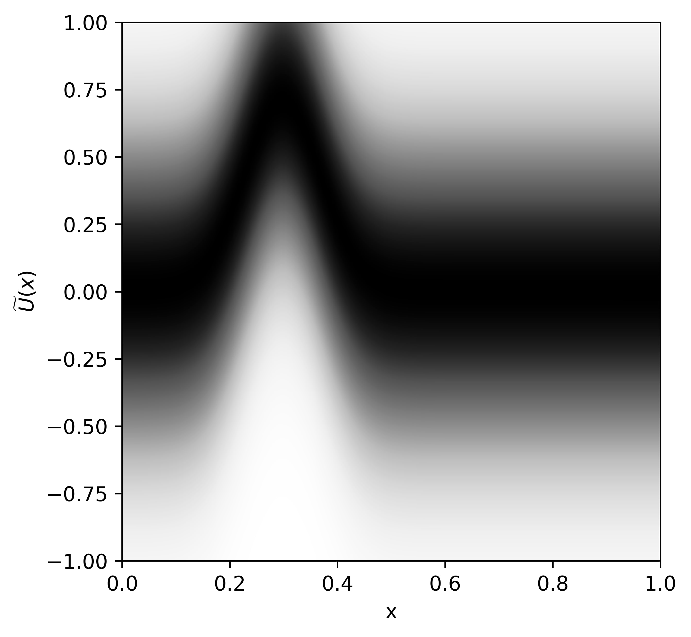
Each hypothesis is defined by values of $\mu$ and $h$. For each pair ($\mu ,h$) we can have a probability distribution on $(x,\tilde{U}(x\left)\right)$. The formula for each hypothesis is:

$\rho (x,y|\mu ,h)=\frac{1}{\sqrt{2\pi {\sigma }_y}}\exp (-\frac{(y-y_0(x,\mu \left)\right)}{2{\sigma }_y^2})$, where $y_0(x,\mu )=h\exp \left(\frac{-(x-\mu {)}^2}{2{\sigma }_x^2}\right)$

(${\sigma }_x$ and ${\sigma }_y$ are chosen beforehand, and equal 0.07 and 0.2 accordingly). The formula is a bit messy, but essentially it is a function with one peak, blurred with noise. 

We can show all of these hypotheses and the probabilities Veronica is assigning to them on a colormap:

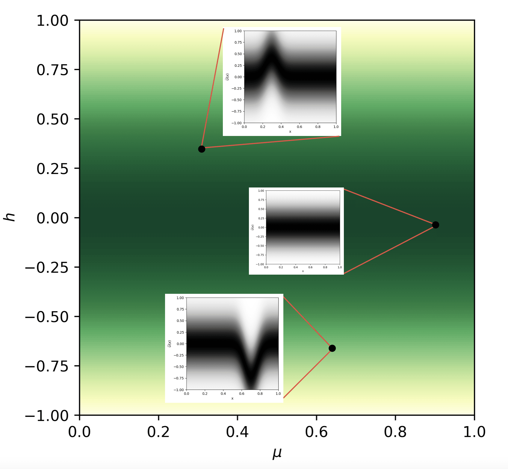
This is Veronica's prior distribution on $(\mu ,h)$-hypotheses. Veronica is skeptical of high peaks, so she puts low prior probability on them. The formula for her prior distribution:

$\rho (\mu ,h)=\frac{1}{\sqrt{2\pi {\sigma }_p}}\exp (-\frac{h^2}{2{\sigma }_p^2})$

(${\sigma }_p$ is the magnitude of her skepticism of high peaks, in our case ${\sigma }_p=1$).

It is worth noting that the actual distribution she gets from the computer is not represented by any hypothesis. But this wouldn't be much of a problem in this setting.

Now Veronica can apply Bayes formula using the observations (in this case, observation is a prediction $(x_i,\tilde{U}(x_i\left)\right)$ she recieves from a computer, in the next formula they would be noted as $(x,y)$).

$\rho (\mu ,h|x,y)=\frac{\rho (x,y|\mu ,h)\rho (\mu ,h)}{P(x,y)}$

She can make updates each time she gets an observation, just like Roman in the previous example.

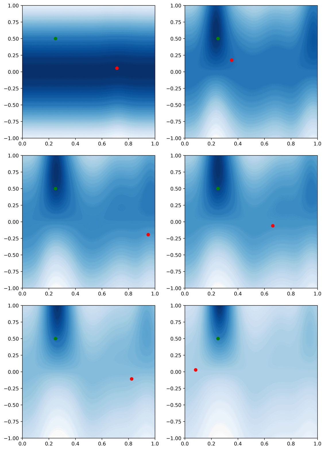
Here is a GIF of a 50 consecutive updates (the red dot represents the observation, and the green dot represents the hypothesis that is closest to the actual distribution we get from the computer):

After this process, Veronica can take the most likely hypothesis and use its $\mu$ value as her best guess for when to sell stocks. Here's her algorithm:

Algorithm 3

1. Set some prior distribution  ${\rho }_0(\mu ,h)$
2. Get the observation $(x_i,\tilde{U}(x_i\left)\right)$ of a prediction from a computer.
3. Calculate posterior distribution using Bayes theorem: ${\rho }_i(\mu ,h|x_i,y_i)=\frac{{\rho }_i(\mu ,h)\rho (x_i,y_i|\mu ,h)}{P(x_i,y_i)}$

4. Set this posterior distribution as new prior distribution and go to step 2. Repeat N times.

   ${\rho }_{i+1}(\mu ,h)={\rho }_i(\mu ,h|x_i,y_i)$

5. Get the most likely hypothesis from last distribution and sell stocks at ${\mu }_{max}$.

   ${\mu }_{max}=\underset{x_i\in [0,1]}{\mathrm{argmax}}\left[{\rho }_N\right(\mu ,h\left)\right]$

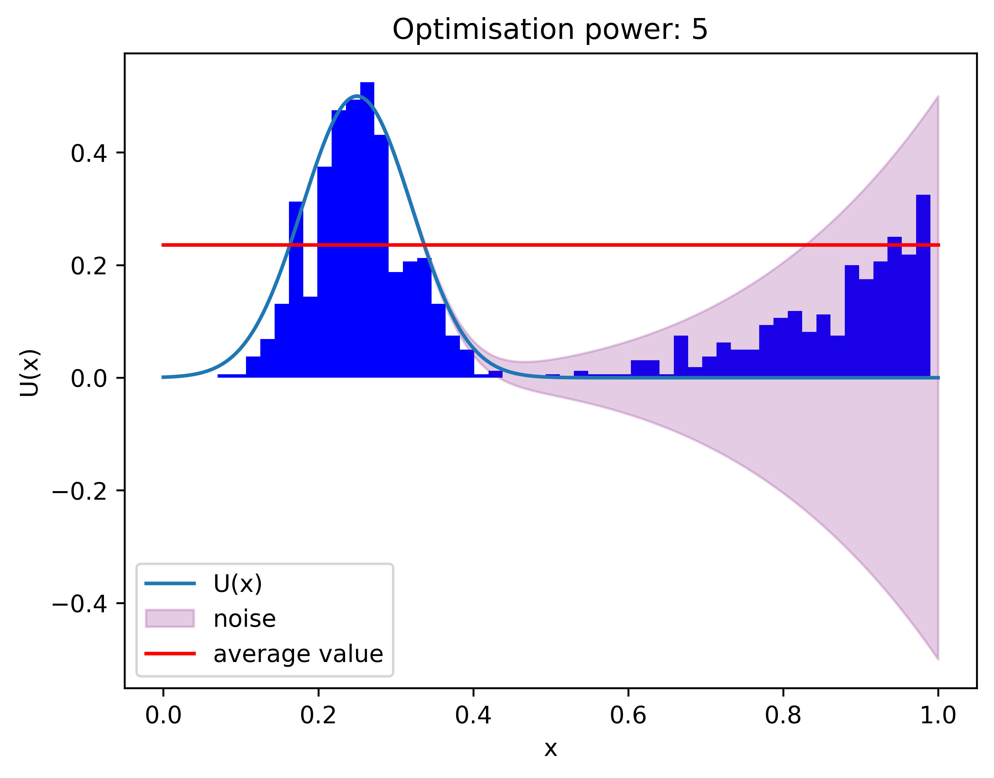
Here is the distribution of these values with 5 updates.

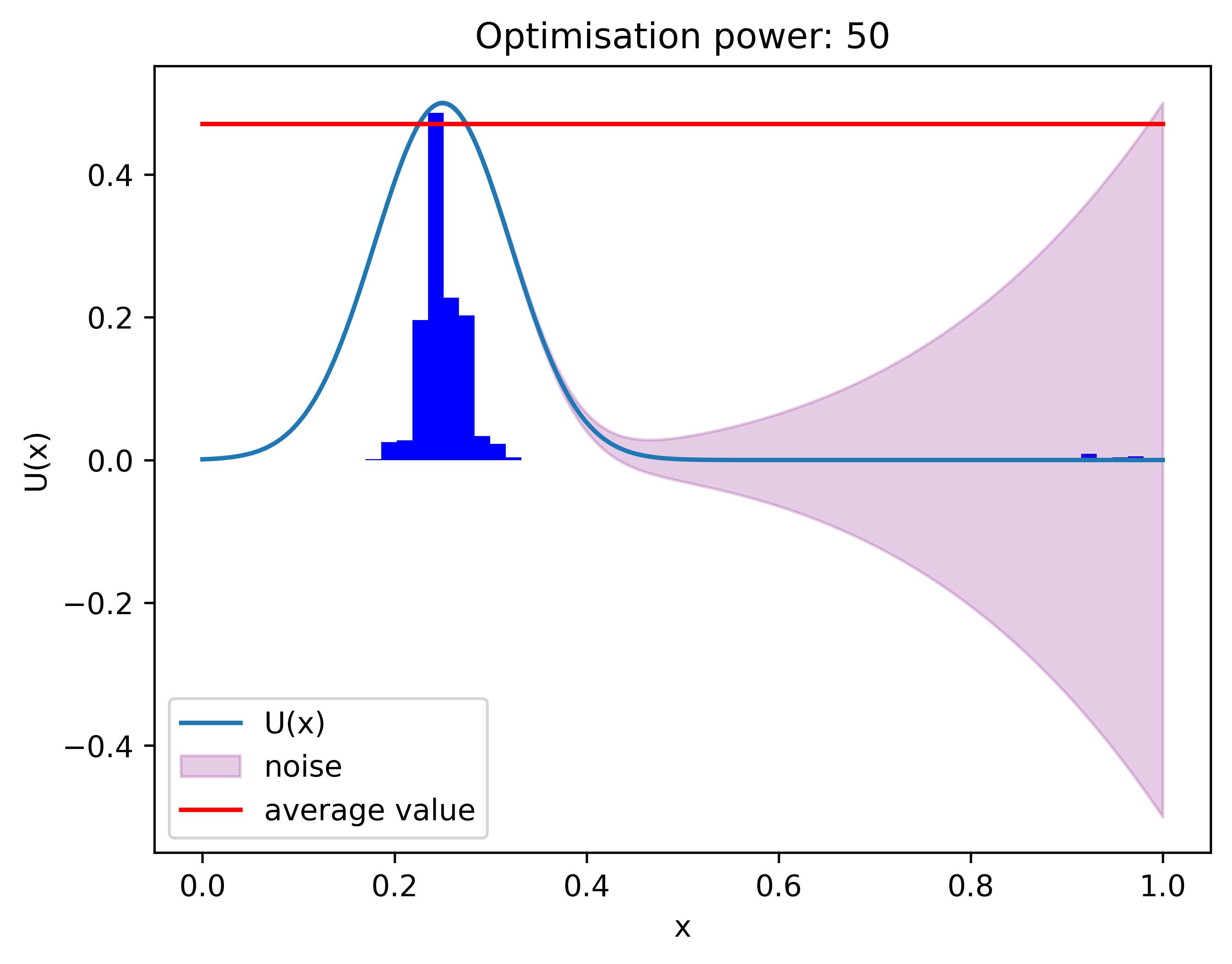
And here is the distribution with 50 updates.

And here is the graph of the average value depending on the number of updates.

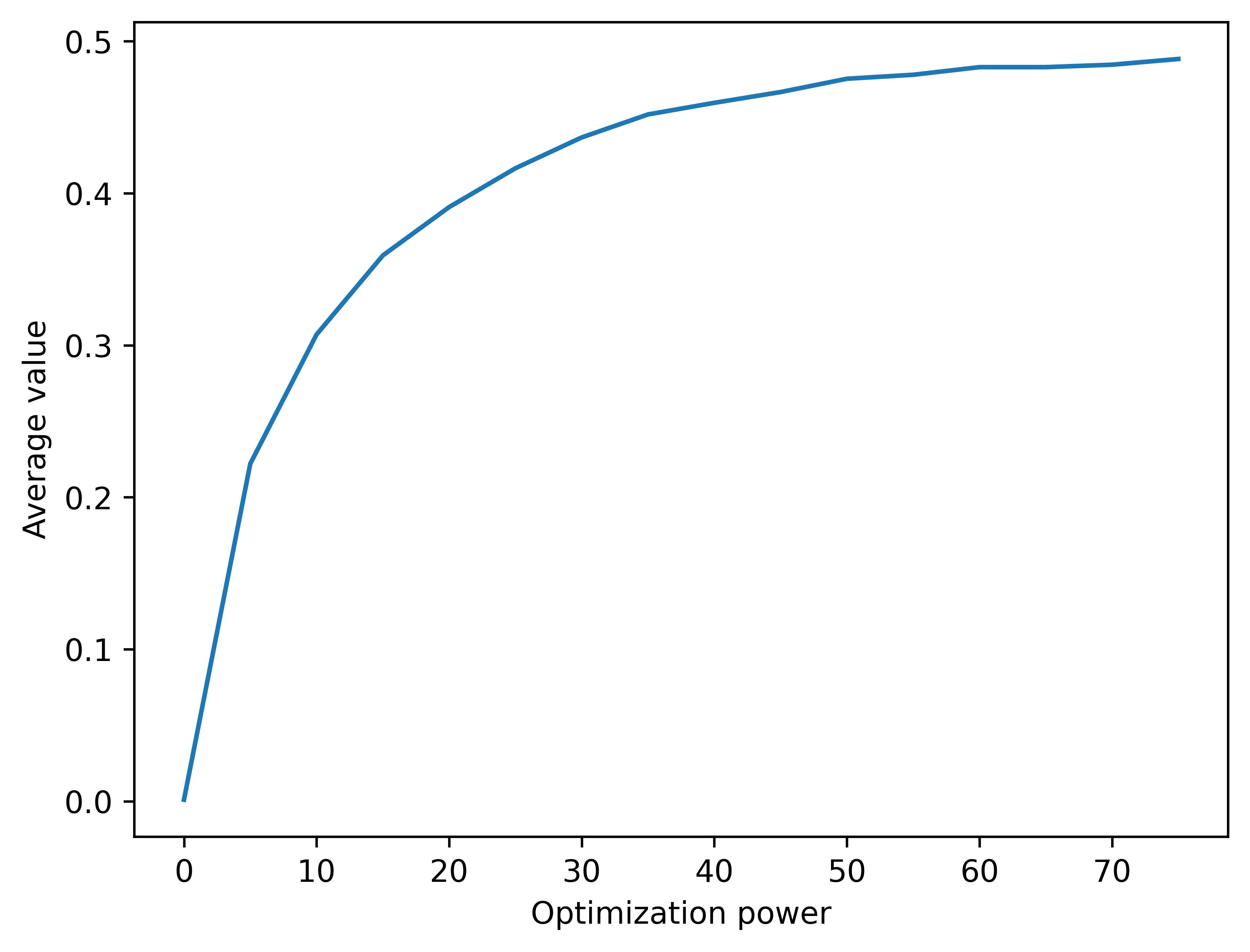
This graph is now again monotonic. Optimizer's curse is cured with Bayesian remedy.

Optimizator's curse arises not only with the kind of optimizator I showed here. It could also be a problem with SGD and other optimizers.

Chapter 4: Goodhart's curse

Now I want to ask a question I had while reading the course materials. Here’s a quote from a post on Goodhart's Curse:

 

Even if $U$ is locally an unbiased estimator of $V$, optimizing $U$ will seek out what we would regard as "errors in the definition", places where $U$ diverges upward from $V$. Optimizing for a high $U$ may implicitly seek out regions where $U-V$ is high; that is, places where $V$ is lower than $U$. This may especially include regions of the outcome space or policy space where the value learning system was subject to great variance; that is, places where the value learning worked poorly or ran into a snag.

Now here is my question: if $V$ is unbiased estimator of $U$ (that is, if we sample a lot of $V_i\left(x_0\right)$ for some fixed $x_0$ and average them out, we get ${\sum }_{i=1}^N\frac{1}{N}{V}_i\left(x_0\right)=U\left(x_0\right)$), what do we mean by $U-V$? If we mean  $E[U-V]$ (expected value), than this is is 0 everywhere, if we mean the random variable $U-V$, then what do we mean by areas where it is high?

1. ^{^}

   Note that this is not a realistic graph of how much money Veronica would make if she sold some stock, this function is chosen for ease of demonstration.

2. ^{^}

   The probability density of distributions is not to the scale on y-axis, I scaled them down so everything would fit in one plot.

3. ^{^}

   The formula for Bayes theorem is as follows:

   $P\left(A|B\right)=\frac{P\left(B|A\right)P\left(A\right)}{P\left(B\right)}$

   For explanation for what each of these terms means, refer to this post [LW · GW], or this post [LW · GW], or this video. I will assume you understand it.

4. ^{^}

   Where $1_A\left(x\right)$ is an indicator function

0 comments

Comments sorted by top scores.