Monosemanticity & Quantization

post by Rahul Chand (rahul-chand) · 2024-10-22T22:57:53.529Z · LW · GW · 0 comments

Contents

  Introduction
  Formulation
  Experiment Details
  Experiments 
  Insights
    How many of our features are active? Here, lesser the better
    What can we learn? 
  Quantization
  Results on Quantization (8-bit)
    Full precision vs. 8-bit
  Results on Quantization (4-bit)
    4-bit vs Full precision
  How do features actually change?
  Additional Thoughts
  Larger models
None
No comments

In this post, I will cover Anthropic's work on monosemanticity^[1]. Starting with a brief introduction to the motivation and methodology. Then move on to my ablation experiments where I train a sparse autoencoder on "gelu-2l"^[2] and its quantized versions to see what insights I can gain.

 

Introduction

The holy grail of mech interpretability is to figure out what feature each single neuron in the network corresponds to and how changing these features changes the final output. Turns out this is really tough because of polysemanticity, that is neurons end up learning/activating for a mixture of features, which makes it tough to find out what exactly does a particular neuron do. One reason this happens is because of "superposition" where the features in a training data are sparse and much more than the number of neurons, therefore, to effectively learn each neuron ends up learning a linear combination of features. 

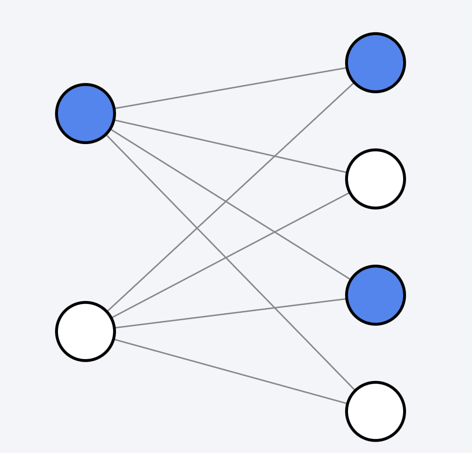
Polysemanticity means it difficult to make statements about what a neuron does. Therefore, we train a sparse autoencoder on top of a already trained neural network which offers a more monsemantic analysis. By that what we mean is, we first hypothesize that each neuron is learning some linear combination of features, these features are more basic and finer grained. Next, if we can figure out what these features are and what feature each neuron activates then we can comment about what task or set of tasks each neuron performs/captures. 

Formulation

Formally, we have a set of basic features $d_i$ (which is larger than the number of neurons) and we attempt to decompose our activations into these directions/features/basis vectors. That is,

                                                            $x_i=b+\sum f_i\left(x^j\right)d_i$ 

where $x_i$ is the output of neuron $i$, $f_i$ is how much the feature $i$ is activated and $d_i$ is a $d$ dimensional vector (same as $x_i$) representing that feature. So, for example, assume there is a feature called "math symbol" and it fires whenever $x_j$ (representation of $j^{th}$ token) corresponds to a term in a math equation ("=", "+", .... etc). $f_i\left(x_j\right)$ is a scalar value which can be 0.9 (if it is a math symbol) and $1e^{-}8$, if it is a normal language non-math token. The original representation $x_i$ is a linear combination of its features. So, a term like "+" might be 0.9*(math symbol) + 0.1*(religious cross). This example is really simplified and in reality, the activations are smaller, and the features finer. 

We have already talked about how the number of features is larger than number of neurons and how each neuron is a linear sum of its features. Therefore, to learn these features and the activations we use sparse dictionary learning, that is 

We have $W_{enc}$ and $b_{enc}$ that takes us from neuron to feature 

                              $f\left(x\right)$ = ReLU($W_{enc}\ast x$ + $b_{enc}$) , where $W_{enc}=(d_f,d)$ 

$d$ = MLP dimension, $d_f$= feature dimension. $d_f>d$ and for finer features $d_f>>d$. $x$ is a $(d,1)$ vector (only consider 1 token here, otherwise its $(d,n)$). Output is a $(d_n,1)$ vector representing how much each feature got activated. Number of non-zero values for $f\left(x\right)$should ideally be 1 (perfect monosemanticity), in practice it is sparse but doesn't have exactly 1 zero. $b_{dec}$ is bias of shape $(d_n,1)$

                                                  $x^{\prime }=W_{dec}\ast f\left(x\right)+b_{dec}$

We go back from feature space to neuron space. $W_{dec}$ is $(d,d_n)$. $W_{dec}$ is also the vector of our features. What I mean by this is that if someone asked you what the vector representing feature "math symbol" is then you would go to $W_{dec}$ and pull out the d dimensional vector corresponding to it.

So, our learning loss is

$L=||x^{\prime }-x|{|}^2$   = $||W_{dec}\ast ReLU(W_{enc}\ast x+b_{enc})+b_{dec}-x||$

Now, we also want sparsity in $f\left(x\right)$, so we add a L1 loss term

Final Loss, 

$L=||x^{\prime }-x|{|}^2$$+\lambda ||f|{|}_1$

 

Experiment Details

The paper works with a toy model (it's a 1 layer transformer but only has 1 FFN layer, as opposed to the 2)

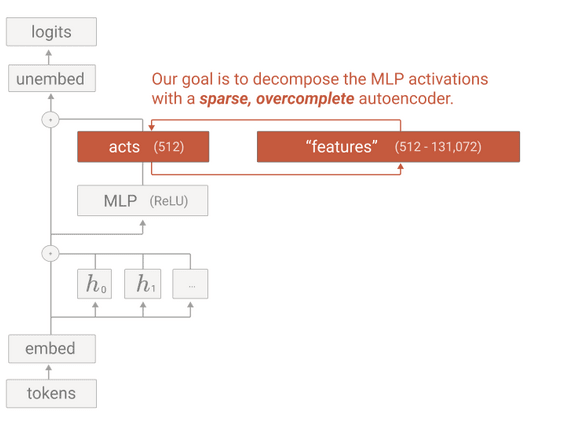
The paper deals with a model made up of only 1 transformer layer (input embedding matrix => self-attention => MLP => output embedding vector). Future work by Anthropic "Scaling Monosemanticity: Extracting Interpretable Features from Claude 3 Sonnet" takes this further and extends the concept to larger practical LLMs^[3]. 

Experiments 

I start with Neel Nanda's github repo on sparse autoencoders^[4] and build over it. The first problem (which is also pointed out by the author) is that it doesn't work out of the box. Therefore, I first fixed the errors in the repo (https://github.com/RahulSChand/monosemanticity-quantization) to allow it work directly out of box. Next, I run a set of experiments, first I train the autoencoder myself and try to see what insights I can gain from seeing the metrics as they train.  For all the below experiments $d_{enc}=32d$. So we are multiplying/zooming 32x (32x more features than neurons)

Insights

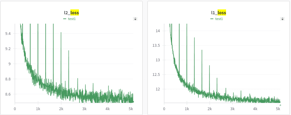
Below is a training plot showing the following metrics

• L2 (reconstruction) and L1 (sparsity) loss

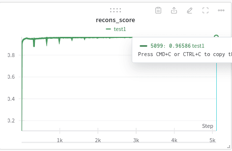
• How close are we to reconstructing original x (as a %)

  

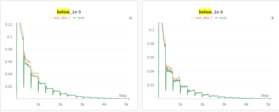
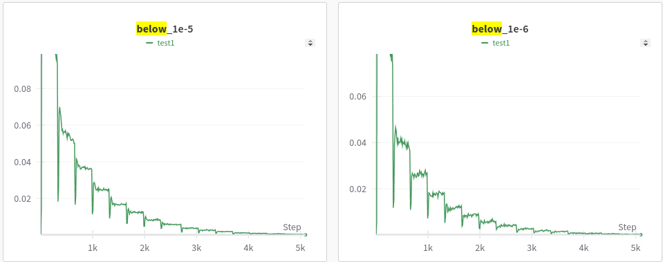
• How many of our features are active? Here, lesser the better

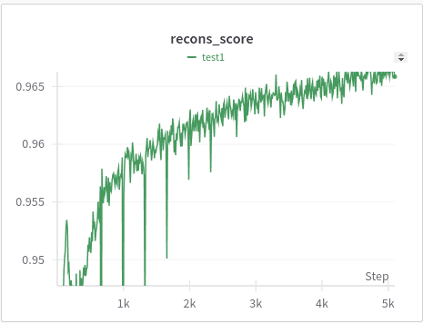
• Plot of reconstruction accuracy (with outliers removed for better viewing)

 

What can we learn? 

First, is that the reconstruction accuracy gets over 90% really quickly (the charts above are for 50% of training data). The reconstruction accuracy is over 90% inside 5% of the training. What does it tell us? Did our sparse autoencoder learn the features so quickly? Seems suspicious, right? Yes, to see what is happening, look at the "below 1e-5 & 1e-6" graphs. Though our reconstruction loss decreases really quickly, we don't learn enough features. Because 20% of our features are below 1e-5, as more data pours in we start to learn more diverse fine grained features. This continues until around we consume 40%-50% of our whole data (even though corresponding L2 and L1 loss are more stagnant). Also, another interesting observation is the "phase transitions", the "below 1e-5" graphs remain stagnant for a while then suddenly have these transitions, as if the model suddenly ends up learning a whole new set of finer features. This is related to so many of phase transitions that we see in LLMs (i.e. at some point the model suddenly becomes much better). 

Another thing to note is that each "phase transition" is accomponied by a sharp loss in reconstruction accuracy (recons_score plot with sharp drops), which points to a sudden increase/change in features => resulting in the model losing accuracy => the model then recovers and finds a way to represent the neurons using this new set of basis features. 

---

Quantization

Next, I run ablation experiments to see how quantization affects these features (Do my features stay the same? Does my sparse autoencoder converge faster? Does it lose features?). I feel this is an interesting direction because many modern LLMs that are served over APIs are quantized version of the full weights, e.g. most Llama API providers serve 4 or 8 bit quantized versons rather than full fp16 weights. Similarly, there are rumors of gemini-flash and gpt-4-mini being 4/8-bit versions of their full precision counterparts. Secondly, quantization being the de-facto way to compress models, I find it interesting that most comparisons of which quantization methods are good or bad involve just results on the final metric & even then many competing quantization (AWQ, GPTQ) give similar performance on metrics. Which one is better? Can we develop a better framework? What if we looked at what "knowledge" is lost when we quantize and what kind of knowledge is lost by different quantizations? I say "knowledge" in quotation marks because it's hard to quantify it, one proxy of knowledge results on benchmarks (which is already used), the other could be what features are lost when we quantize (in which case we could use methods like monosemanticity to study them).

Results on Quantization (8-bit)

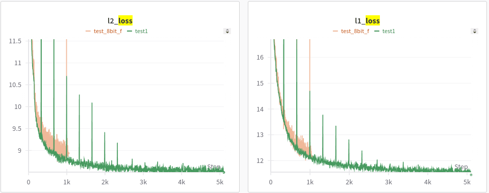
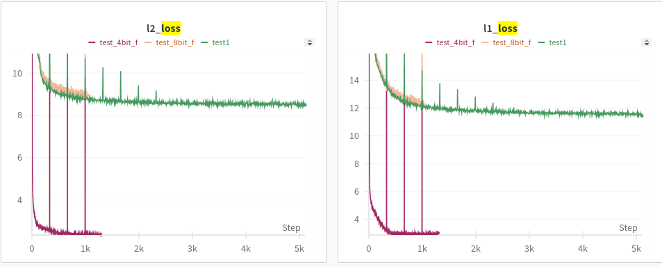
• L2 and L1 loss

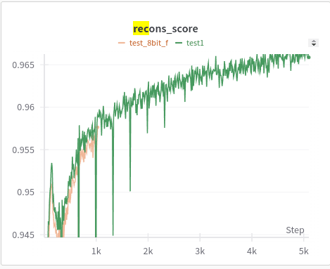
• Reconstruction accuracy

• below 1e-5 & 1e-6

• 

 

Full precision vs. 8-bit

What do we learn from the above? First, is that the learning trend is similar (fast convergence of L2, phase transition and slower convergence of how many features are active). And as expected the 8-bit reconstruction accuracy is slightly behind full precision and similarly the number of features that are active is also slightly behind. This is in line with what we know already, 8 bit makes the model worse but it's not that bad. For most LLMs int8 and fp16 are very close. A better analysis here would be to look at specific features (which I try to cover in a later section)

Results on Quantization (4-bit)

• L1 & L2. Why is 4-bit L2 and L1 so good?

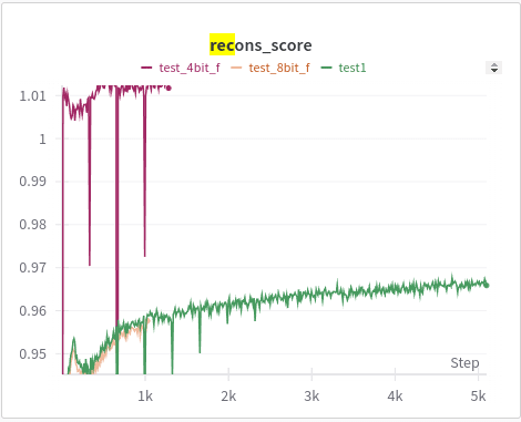
• reconstruction accuracy. why is it reconstruction so good?

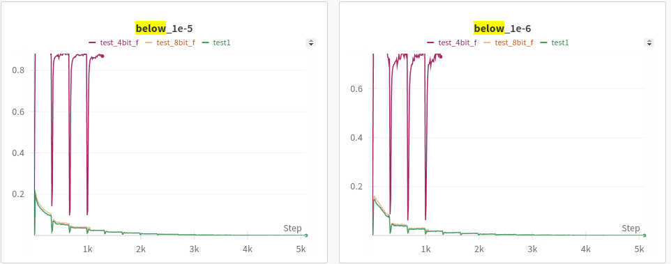
• below 1e-5 & 1e-6

 

4-bit vs Full precision

Few things happened as expected, the quant 4 model was so bad that that its activations are almost noise which means that the reconstruction accuracy, which is how good is our model when it is fed x vs. when it is fed x' is high. Because when you feed it x (the activations of the 4-bit quantized model with no sparse autoencoder) then the results are already really bad and the results remain bad when you feed it x'. It's like comparing garbage against garbage even if they are close, it tells us nothing. Other interesting thing is that the L2 and L1 loss are much lower, our sparse autoencoder learns to very accurately map x to x' but the "below_1e-5/1e-6" plots show that it doesn't learn any features while doing so, more than 80% of features are below 1e-5. It is as if it just zeros out a lot of features (which reduces L1) and just maps x to x' without learning any features. 

Confusion about L1 loss vs. "below 1e-5". L1 loss = sum of values in a vector. "below 1e-5" = how many features are more than >0 on average. You can get low L1 but high "below 1e-5" if you only have a very small set of features always highly active (as is happening in the degenerate case of 4-bit where model only activates the SAME set of features for all points)

 

How do features actually change?

Below I plot, how many features are active across 50 batch examples. This is the log of the frequency, so if a feature is on the right, it means its activated more times than a feature on the left.

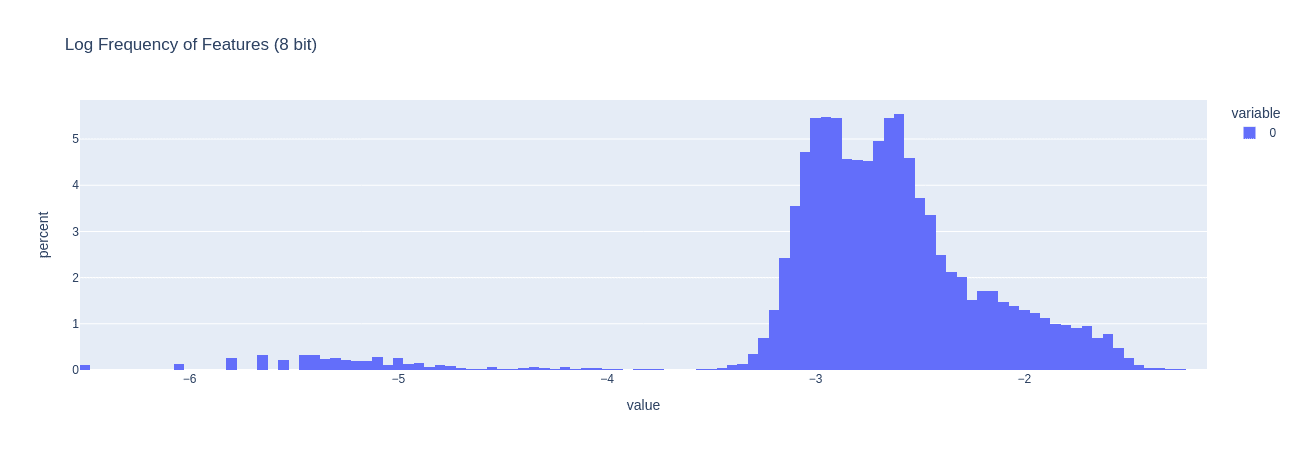
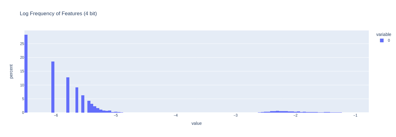
A better experiment to check how features change would be to

1. Get a model and its quantized versions
2. Train the encoder for all of them
3. For each of the encoder make a large list of features and see if there are features missing in 8-bit or 4-bit models

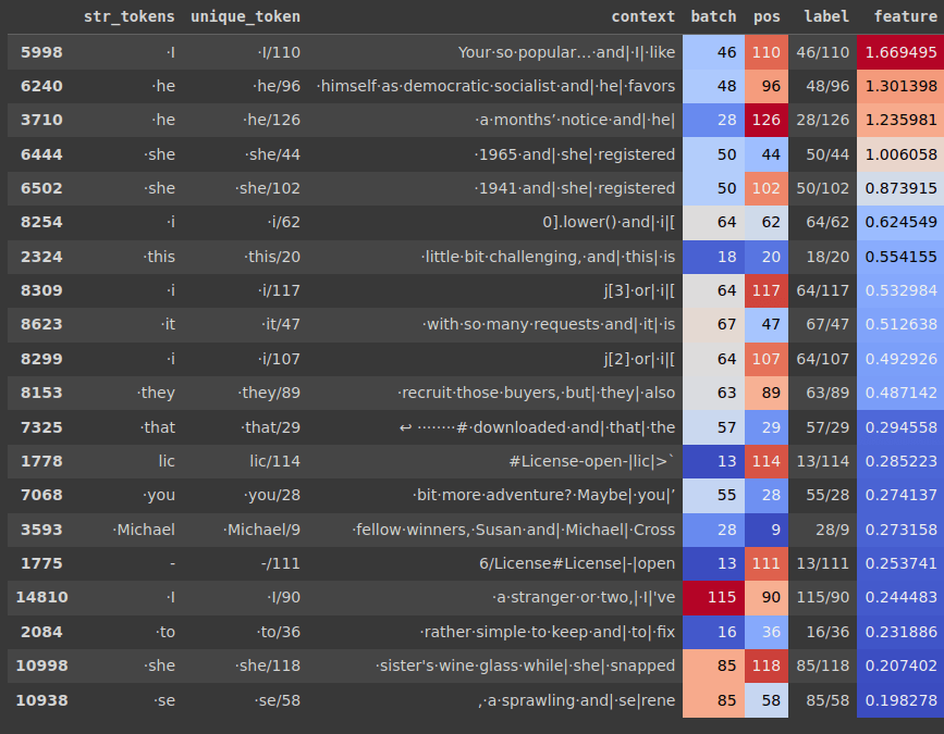
This experiment would take time because once you find a feature in a model, you cannot be sure if the same feature occurs at the same position in the other model's autoencoder. The other experiment we can do is to find examples from a batch which activate a certain feature $i$ in a model, then pass these examples into the other model and see if we can isolate a feature $j$ which activates primarily for the selected input examples. 

Additional Thoughts

In my opinion the issue with methods like these is that you can find patterns where there are none. This is something that has already been pointed out by others. More specifically going over this great blog post^[5] gave me some of the ideas that I am going to discuss next

• First, from what I understand looking at the code and paper, the way we find interpretable features is we pick a feature (we don't know the meaning of that feature yet, only that it is the $i^{t}h$ feature). Then we pass in a bunch of text tokens and see for which text tokens does this feature consistently remain high. Finally, we make a connection between the feature and the text tokens we see. In some cases, this can work really well, if all the tokens that activate your feature are math tokens then this feature is related to math symbols. But for other features, the ones we are more interested in, e.g. related to safety (like "bioweapon" or "gore" etc.) its hard to know what we are looking at. We will need to do a guess work. For e.g. if you see a feature that gets activated for tokens related to bioweapons then is it because that feature encodes "bioweapon" or is it just firing when it sees some certain combination of work like "bio & pon". This is where we see patterns because we want them to be
• The second issue is that this method doesn't allow us to directly find features of interest. It works in the opposite direction. You sift through all features then you assign them meaning and then you try to see if the feature you are interested is in exists or not.

"This work does not address my major concern about dictionary learning: it is not clear dictionary learning can find specific features of interest, "called-shot" features [LW · GW], or "all" features (even in a subdomain like "safety-relevant features"). I think the report provides ample evidence that current SAE techniques fail at this"

• Third, as pointed out by the blog, a feature isn't its highest activating examples

"I think Anthropic successfully demonstrated (in the paper and with Golden Gate Claude) that this feature, at very high activation levels, corresponds to the Golden Gate Bridge. But on a median instance of text where this feature is active, it is "irrelevant" to the Golden Gate Bridge, according to their own autointerpretability metric! I view this as analogous to naming water "the drowning liquid", or Boeing the "door exploding company". Yes, in extremis, water and Boeing are associated with drowning and door blowouts, but any interpretation that ends there would be limited."

 

Larger models

For larger models we move away from focusing on MLP to focus on the residual stream since when working with larger models (with multiple layers) features tend to diffuse into multiple layers and the activations of 1 layer don't correspond to concrete features. In the github repo, I have added ways to run experiments similar to the ones in the follow up paper (using residual streams and additional losses). 

 

1. ^{^}

   https://transformer-circuits.pub/2023/monosemantic-features/index.html

2. ^{^}

   https://huggingface.co/NeelNanda/GELU_2L512W_C4_Code

3. ^{^}

   Briefly covered in the "Larger Models" section at the end

4. ^{^}

   https://github.com/neelnanda-io/1L-Sparse-Autoencoder

5. ^{^}

   https://www.lesswrong.com/posts/zzmhsKx5dBpChKhry/comments-on-anthropic-s-scaling-monosemanticity

0 comments

Comments sorted by top scores.