Part 1: Enhancing Inner Alignment in CLIP Vision Transformers: Mitigating Reification Bias with SAEs and Grad ECLIP

post by Gilber A. Corrales (mysticdeepai) · 2025-02-03T19:30:52.505Z · LW · GW · 0 comments

Contents

  Abstract:
  1. Introduction
    1.1. Presentation of the CLIP Model and Its Relevance in Multimodal Systems
    1.2. Importance of Interpretability in Advanced Models
    1.3. Problem Statement
  2. Definition and theoretical foundations
    2.1. Defining the CLIP Model with a Mathematical Foundation
    2.2. Introduction to Sparse Autoencoders and the Jumped SAE Configuration
    2.3 Inner Alignment and Transparency 
  3. Methodology
    3.1 Training of SAEs
    3.2  Analysis of SAEs
  4. Results
    4.1 Evolution of Metrics over Training Steps
  5. Conclusion
None
No comments

Abstract:

In this work, we present a methodology that integrates mechanistic and gradient-based interpretability techniques to reduce bias in the CLIP Vision Transformer, focusing on enhancing inner alignment. We begin by defining the CLIP model and reviewing the role of Sparse Autoencoders (SAEs) in mechanistic interpretability, specifically highlighting the use of the Jumped SAE configuration. We then introduce Grad ECLIP—a gradient-based method tailored for CLIP—to visualize the model’s focus areas. We apply our approach to detect and mitigate the reification bias associated with sexual objectification in CLIP, wherein the model disproportionately focuses on certain visual features (specifically, the bust region in images of semi-nude women). Using the Sexual OBjectification and EMotion (SOBEM) dataset of 280 images (140 images of semi-nude women and 140 images of the same women wearing a shirt), we extract residual activations from layers 22, 23, and 24 of the CLIP Vision Transformer, train nine different SAEs with expansion factors of x8, x16, and x32, and select the most appropriate SAE based on statistical evaluation. By integrating the selected SAE into CLIP and analyzing the resulting Grad ECLIP heatmaps—evaluated via Intersection over Union (IoU) with manually created bust masks—we test whether our intervention successfully reduces the bias. Finally, an ablation strategy is applied to validate the causal impact of our intervention on bias reduction and to improve the model’s inner alignment.

Link of implementation: https://github.com/MysticDeepAI/HeatMapSae-A-Gradient-Centric-Approach-to-Explaining-CLIP-Through-Sparse-Latent-Activations

1. Introduction

1.1. Presentation of the CLIP Model and Its Relevance in Multimodal Systems

The CLIP (Contrastive Language–Image Pre-training) model  (Radford et al)represents a significant advancement in multimodal systems by jointly embedding images and textual descriptions into a shared latent space. Developed to bridge the gap between visual and textual data, CLIP utilizes a Vision Transformer (ViT) architecture, which has shown remarkable performance in various computer vision tasks. Its ability to understand and relate concepts across modalities makes it a powerful tool in contexts ranging from image retrieval to content moderation. However, the complexity and high dimensionality of its internal representations pose challenges for both transparency and accountability, especially as these models are increasingly deployed in real-world, high-stakes applications.

1.2. Importance of Interpretability in Advanced Models

Interpretability is a cornerstone of responsible AI development, particularly for systems with far-reaching societal impacts. In advanced models like CLIP, understanding the decision-making process is essential not only for building trust among users but also for identifying and mitigating biases that could lead to unfair or harmful outcomes. Mechanistic interpretability techniques have emerged as a promising avenue to dissect the internal workings of such models. Among these techniques, Sparse Autoencoders (SAEs) have been effectively used to decompose complex activations into a set of sparse, interpretable features. In our work, we leverage the Jumped SAE configuration proposed by (Lieberum et al) in Gemma Scope—a specific variant that has demonstrated strong performance in isolating discrete, meaningful features—to facilitate a clearer understanding of CLIP’s internal processes.

1.3. Problem Statement

Despite CLIP’s impressive capabilities, its internal activations can inadvertently encode harmful biases that influence model behavior. In our study, we leverage the Sexual Objectification and Emotion (SOBEM) database—a standardized and controlled picture dataset specifically designed to study sexual objectification (Ruzzante et al.)—to investigate these issues, focusing on a reification bias in which the model disproportionately attends to certain visual features—most notably, the bust region in images of semi-nude women. This bias not only distorts the model’s attention but also reinforces harmful stereotypes by de-emphasizing human characteristics such as emotional expression in objectified individuals (Wolfe et al.). Such misrepresentations indicate a misalignment between the model’s internal representations and the desired equitable and transparent behavior. Therefore, identifying and decomposing these internal activations is critical for understanding the roots of this bias and for designing targeted interventions. Ultimately, this deeper insight is essential to mitigate the impact of sexual objectification in vision-language models and to enhance their overall inner alignment.

2. Definition and theoretical foundations

2.1. Defining the CLIP Model with a Mathematical Foundation

CLIP (Contrastive Language–Image Pre-training) is a multimodal model designed to jointly learn visual and textual representations from large-scale web-curated image–text pairs. At its core, CLIP consists of two encoders—a vision encoder  $I(\cdot )$  and a text encoder  $T(\cdot )$ —which map images and text into a unified embedding space. The goal is to ensure that corresponding image–text pairs have similar representations while non-corresponding pairs are pushed apart.

Given an image–text pair $(I,T)$, the encoders produce feature embeddings $f_I\in R^D$  and $f_T\in R^D$, respectively. The matching score  S  between the image and text is defined as the cosine similarity between these embeddings:

 

$$S(f_I,f_T)=\cos (f_I,f_T)=\frac{f_I\cdot f_T}{\parallel f_I\parallel \parallel f_T\parallel }$$

This score is used within a contrastive learning framework where true image–text pairs are treated as positive examples, and mismatched pairs as negatives.

A key component of the vision encoder is its transformer architecture, which processes an image by first dividing it into patches and then projecting these patches into a sequence of tokens. Notably, the model prepends a special class token [CLS] to the sequence. The final image representation $f_I$  is typically derived from the output corresponding to this class token.

More specifically, the attention mechanism within the transformer plays a crucial role. For the class token, the output of an attention layer can be expressed as:

 

$$o_{\text{cls}}=\sum _i\text{softmax}\left(\frac{q_{\text{cls}}^{\top }{k}_i}{\sqrt{C}}\right)v_i$$

where:
-  $q_{\text{cls}}$ is the query vector for the class token.
-  $k_i$  and $v_i$  are the key and value vectors corresponding to the  i -th image patch.
-  $C$  is the channel dimension, and the softmax operation normalizes the weights across all patches.

The final image embedding is then obtained by applying a linear projection  $\text{LP}(\cdot )$  to the class token’s output:
 

$$f_I=\text{LP}\left(o_{\text{cls}}\right)$$

This formulation highlights how CLIP aggregates spatial information from various patches into a single vector that captures high-level, discriminative features. The transformer’s layered structure further refines these representations, with layers 22, 23, and 24 often containing rich, abstract features essential for downstream tasks and interpretability.
 

2.2. Introduction to Sparse Autoencoders and the Jumped SAE Configuration

Sparse Autoencoders (SAEs) are an unsupervised technique for decomposing a neural network’s internal activations into a sparse, linear combination of interpretable feature vectors. Formally, given an activation $x\in R^n$  (for instance, obtained from a Vision Transformer like CLIP), an SAE is composed of two functions:

Encoder

$$f\left(x\right)=\sigma (W_{\text{enc}}x+b_{\text{enc}})$$

where $W_{\text{enc}}$  and $b_{\text{enc}}$ are the encoder’s parameters, and $\sigma$ is an activation function that, together with appropriate regularization, encourages sparsity in $f\left(x\right)$.

Decoder
 

$$\hat{x}=W_{\text{dec}}f\left(x\right)+b_{\text{dec}}$$

The goal is to reconstruct the input $x$ as accurately as possible by minimizing a loss function that combines the reconstruction error (often measured by the mean squared error) with a sparsity penalty (typically imposed using an  $L_0$  or  $L_1$ norm).

In our work, we adopt the Jumped SAE configuration, which is based on the JumpReLU activation function. This approach enhances sparsity by introducing an adaptive threshold. Instead of using the standard ReLU function, JumpReLU is defined as:

 

$$\sigma \left(z\right)={\text{JumpReLU}}_{\theta }\left(z\right):=z\odot H(z-\theta )$$

Here:
-  $z$  is the pre-activation vector.
-  $\theta$  is a learnable threshold vector with  $\theta >0$.
-  $H(\cdot )$  is the Heaviside step function, which outputs 1 if its argument is positive and 0 otherwise.
-  $\odot$ denotes elementwise multiplication.

This gating mechanism ensures that only those components of  $z$  that exceed the threshold  $\theta$ are allowed to pass through, effectively forcing the activation  $f\left(x\right)$ to be sparse. By decoupling the selection of active latents (via thresholding) from the estimation of their magnitudes, the JumpReLU SAE configuration yields a representation that is both sparse and more interpretable. Additionally, it allows a variable number of latents to be active per token, which is particularly valuable for transformer models where the complexity of activations can vary significantly.

In our project, we leverage Jumped SAEs to decompose the residual activations extracted from layers 22, 23, and 24 of the CLIP Vision Transformer. This configuration is chosen for its demonstrated ability to isolate meaningful internal features, thereby aiding in the detection and mitigation of biases—such as the reification bias that causes the model to disproportionately focus on the bust region in images of semi-nude women. Moreover, this approach contributes to enhancing the inner alignment of the model by ensuring that its internal representations more closely align with fair and transparent behavior.

2.3 Inner Alignment and Transparency
 

Understanding the inner alignment of a model is critical for ensuring that its internal representations and decision-making processes are consistent with its intended behavior. By interpreting the activations within the network—specifically, through techniques such as Sparse Autoencoders and gradient-based methods—we gain insight into the latent features that drive predictions. This deep examination of internal activations not only reveals how different components contribute to the final output but also highlights potential misalignments or biases within the model. In turn, such interpretability enhances the overall transparency of the system, enabling developers and researchers to identify, understand, and correct discrepancies between the model’s internal workings and the desired ethical and performance standards.

 

3. Methodology

3.1 Training of SAEs

In our study, we first extracted the residual activations from the final three residual layers (layers 24, 23, and 22) of the CLIP Vision Transformer for a curated dataset of 280 images. These images comprise 140 images of semi-nude women and 140 images of the same women wearing a shirt, each paired with a prompt that reflects the sentiment inferred from their facial expressions. These activations serve as the input for our Sparse Autoencoder (SAE) training. 

We implemented our SAE using a JumpReLU configuration, which enhances sparsity by employing an adaptive threshold mechanism. To assess the impact of model capacity on sparsity and reconstruction performance, we trained nine distinct SAEs using three different expansion factors: x8, x16, and x32. The training was conducted over 10,000 steps (not epochs), during which we monitored key metrics such as the L0 norm (the average count of non-zero latent activations per batch), the Fraction of Variance Unexplained (FVU) as a measure of reconstruction fidelity, the reconstruction loss (measured using mean squared error), and the total loss (a sum of reconstruction and sparsity penalties). 

The L0 metric quantifies the sparsity by counting the number of latent activations greater than zero, while FVU provides an estimate of the variance not captured by the reconstruction relative to a baseline prediction of the batch mean. This systematic training procedure, grounded in a mathematically rigorous framework, enabled us to select the optimal SAE configuration based on a thorough statistical evaluation, thereby laying the foundation for our subsequent analysis using gradient-based techniques.

3.2  Analysis of SAEs

In this phase, we conducted a comprehensive analysis to evaluate the performance of our trained SAEs, identify the optimal configuration for our application, and detect candidate neurons associated with bias. First, we generated Sparsity vs. Fidelity graphs that compared all autoencoder configurations using the $L0$ metric  and the reconstruction loss. We then analyze the final values ​​of all the extracted metrics.

To further investigate the latent representations, we computed the average histogram of activations for each neuron in the SAE latent space. Each activation was classified based on the image labels—distinguishing between images of semi-nude women and those of women wearing a t-shirt. To enhance visibility, we applied a logarithmic transformation, $\log (1+x)$ , to the activations. We subsequently subtracted the average activations of the two classes to identify candidate neurons that could encode the bias of interest.

Dimensionality reduction was then performed on the latent activations using Principal Component Analysis (PCA) to project the data into two dimensions. We employed K-means clustering, guided by both the silhouette score and the elbow method, to group the reduced data, and each PCA point was annotated with its corresponding label (semi-nude or wearing a t-shirt).

To determine the optimal layer and expansion factor that best capture the bias, we applied statistical tests including the Kolmogorov-Smirnov Test and the Mann–Whitney U Test. These tests helped us identify the layer and SAE expansion factor that exhibited the most significant differences between the two image groups in terms of both the mean activation values and their distributional shape. We further quantified the magnitude of these differences using Cliff's Delta to obtain a matrix representing the level of divergence between groups.

Finally, we evaluated the effect of integrating the SAEs by comparing the cosine similarity of the CLIP model's outputs with and without the SAE processing across all 280 images.

 

4. Results

4.1 Evolution of Metrics over Training Steps

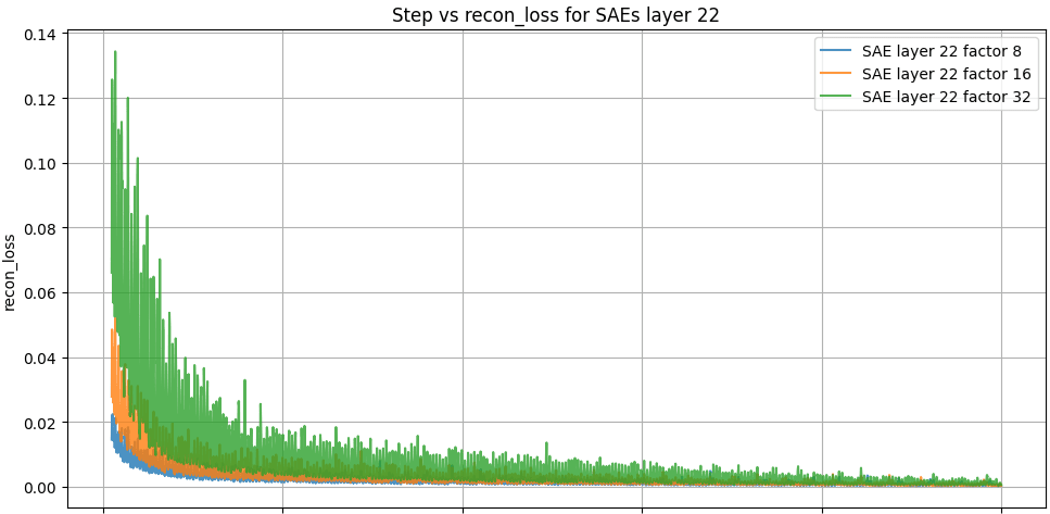
The Figure 1 "Step vs recon_loss for SAEs layer 22" provides critical insights into the performance of Sparse Autoencoders (SAEs) trained with different expansion factors (x8, x16, x32). All configurations demonstrate a significant reduction in reconstruction loss during the initial training steps, indicating effective learning of the residual activations. The x8 expansion factor achieves the lowest reconstruction loss, suggesting superior reconstruction fidelity, while larger factors (x16 and x32) exhibit higher initial losses and greater variability, though they eventually converge. The final plateau in reconstruction loss highlights potential architectural or sparsity-regularization constraints on the models' reconstruction capabilities. In summary, while lower expansion factors (x8) prioritize precise reconstruction, larger factors (x16 and x32) may better capture complex latent patterns, making them more suitable for identifying critical biases and differences in the dataset depending on the specific research objectives.

 

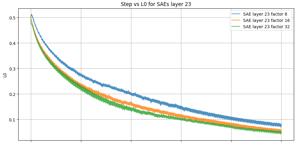
The Figure 2 "Step vs L0 for SAEs layer 23" provides a detailed perspective on the sparsity dynamics across different expansion factors (x8, x16, x32) during training. The L0 metric, which quantifies the average number of active latent units per batch, decreases progressively over training steps for all expansion factors, reflecting the sparse representations encouraged by the loss function. The x8 expansion factor exhibits the highest L0 values, indicating less sparsity compared to x16 and x32, which show progressively lower L0 metrics and, thus, sparser activations. This trend suggests that higher expansion factors (x32) may enforce stricter sparsity constraints, potentially capturing more interpretable latent representations at the cost of reduced reconstruction fidelity.

Interestingly, the behavior of L0 indicates consistent sparsity enforcement throughout training, although with different degrees depending on the expansion factor. Exploring how modifying the sparsity regularization weight $\lambda$ in the total loss function affects this behavior would provide valuable insights. Adjusting λ could influence the trade-off between sparsity and reconstruction fidelity, potentially altering the $L0$ dynamics and the quality of the learned latent representations. Such experiments could help optimize the SAE configuration for specific applications requiring a balance between interpretability and fidelity.

 

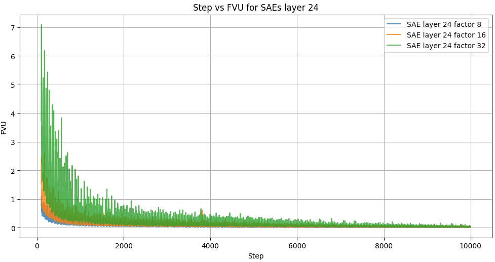
The Figure 3 "Step vs FVU for SAEs layer 24" illustrates the Fraction of Variance Unexplained (FVU) as a function of training steps for Sparse Autoencoders (SAEs) with expansion factors x8, x16, and x32. The FVU metric measures the proportion of variance in the input data not captured by the reconstruction, providing insight into the fidelity of the learned representations.

Across all expansion factors, the FVU decreases significantly during the initial stages of training, indicating rapid improvement in the reconstruction accuracy. The x8 expansion factor achieves the lowest FVU values throughout the training, demonstrating the highest reconstruction fidelity. In contrast, x16 and x32 exhibit slightly higher FVU values, with x32 displaying the largest variability and the slowest convergence. This suggests that larger expansion factors might prioritize sparsity over reconstruction fidelity, resulting in higher unexplained variance but potentially more interpretable representations.

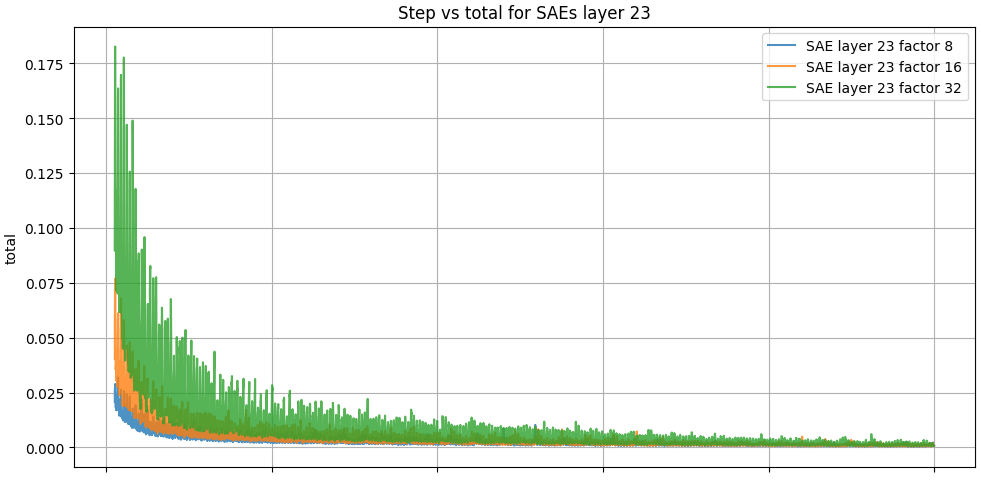
The figure 4 "Step vs total for SAEs layer 23" displays the evolution of the total loss, which combines reconstruction loss and sparsity regularization, across training steps for Sparse Autoencoders (SAEs) with expansion factors x8, x16, and x32. This metric provides a comprehensive measure of the trade-off between reconstruction fidelity and the imposed sparsity constraints during the learning process.

All configurations show a steep decline in total loss during the initial steps, reflecting the rapid optimization of the model as it learns to balance reconstruction accuracy with sparsity. The x8 expansion factor achieves the lowest total loss consistently throughout training, indicating a better trade-off between sparsity and reconstruction fidelity. Meanwhile, x16 and x32 have higher total loss values, with x32 demonstrating the greatest variability during training. This variability is likely due to the more aggressive sparsity constraints imposed by larger expansion factors, which require the model to allocate more capacity to satisfy the sparsity regularization.

The scatter plot in figure 5 "Trade-off: Sparsity (L0) vs. Fidelity (Reconstruction Loss)" illustrates the relationship between the final reconstruction loss (fidelity) and the fraction of active neurons (L0 sparsity) across different SAE configurations and layers. Lower L0 values indicate higher sparsity, while lower reconstruction loss represents better fidelity.

Key insights:

• Layer 22 factor 8 achieves the best reconstruction fidelity but at the cost of lower sparsity.
• Layer 24 factor 32 shows the highest sparsity but with the poorest reconstruction fidelity.
• Configurations with higher expansion factors (e.g., factor 32) generally favor sparsity over fidelity, while lower factors (e.g., factor 8) prioritize fidelity.

This trade-off underscores the importance of selecting the appropriate configuration based on the desired balance between interpretability and reconstruction accuracy.

 

 

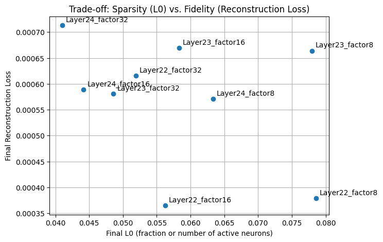
The next table summarizes key metrics for different combinations of layers and expansion factors. Based on all metrics (Reconstruction Loss, L0, FVU, and Total Loss), the best-performing configuration is Layer 22 with factor 16, achieving the lowest Reconstruction Loss (0.000365) while maintaining a good balance in sparsity (L0 = 0.056236), FVU (0.014365), and Total Loss (0.000421). This indicates that this configuration optimally balances fidelity and sparsity for effective representation learning.

Layer	Factor	Steps	Reconstruction loss	L0	FVU	Total Loss
22	16	10000	3.65e-4	5.62e-2	1.43e-2	4.21e-4
22	32		6.16e-4	5.19e-2	2.42e-2	6.68e-4
22	8		3.76e-4	7.85e-2	1.49e-2	4.57e-4
23	16		6.69e-4	5.83e-2	1.87e-2	7.27e-4
23	32		5.81e-4	4.85e-2	1.62e-2	6.30e-4
23	8		6.64e-4	7.79e-2	1.85e-2	7.42e-4
24	16		5.89e-4	4.41e-2	1.47e-2	6.33e-4
24	32		7.13e-4	4.10e-2	1.77e-2	7.54e-4
24	8		5.71e-4	6.33e-2	1.42e-2	6.34e-4

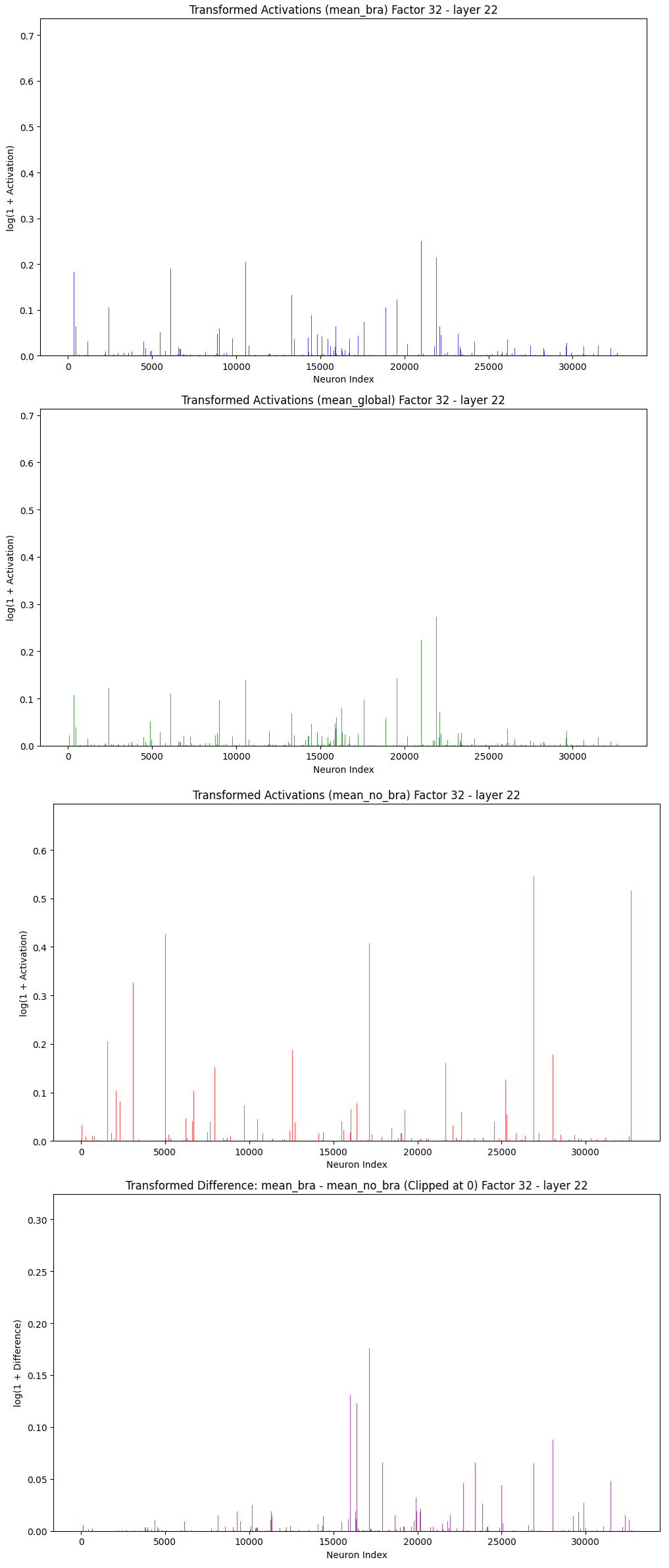
This set of graphs visualizes the average transformed activations for different subsets of images and identifies potential candidate neurons associated with specific features.

• The first three graphs show the average activations for all images (global mean), for images of semi-nude women (mean_bra), and for images of women wearing a shirt (mean_no_bra). These activations are transformed using $\log (1+\text{Activation})$ for better visualization.
• The final graph represents the difference in mean activations between the two subsets (mean_bra - mean_no_bra), with negative values clipped to zero. This highlights candidate neurons that are likely capturing features specifically associated with semi-nude women, as they exhibit higher activations for this subset compared to the shirt-wearing group.

This analysis effectively identifies neurons that might encode biased or specific features, providing a basis for further interpretability and fairness investigations.

 

 

The statistical analysis aimed to identify the layer and factor combinations with the greatest structural differences in activations between two groups: images of semi-nude women and women wearing a shirt. The evaluation was performed using Mann-Whitney $p-values$, effect size $\left(r\right)$, and Cliff’s Delta$\left(\delta \right)$ to determine both statistical and practical significance.

The combination Layer 22, Factor 16 yielded the most notable results, with a highly significant $p-value$$(1.04\times {10}^{-9})$, a large effect size $(r=0.516)$, and a small to moderate practical difference $(\delta =0.032)$. Similarly, Layer 22 and Layer 23 with Factor 32 demonstrated significant differences ($p=7.10\times {10}^{-17}$ and $8.64\times {10}^{-11}$, respectively), with $\delta$ values of 0.030 and 0.024, indicating meaningful structural variations in the activations between the two groups.

In contrast, Layer 24 across all factors showed negligible practical differences $(\delta <0.02)$ despite some statistically significant p-values, suggesting limited relevance for capturing structural differences. Factor 8, Layer 22, while statistically significant $(p=0.0121)$, exhibited only a small practical difference $(\delta =0.019)$.

The selected configurations for further analysis were Factor 16, Layer 22, and Factor 32, Layers 22 and 23, as they exhibited statistically significant differences and practical relevance. These configurations provided the most robust candidates for analyzing disparities in activations between the two groups of images.
 

Factor	Layer	Mann–Whitney $p$	Effect Size $r$	Cliff’s Delta$\left(\delta \right)$	Significant
8	22	1.21e-2	5.10e-1	1.90e-2	Significant
8	23	5.56e-1	5.02e-1	5.00e-3	Not Significant
8	24	5.59e-2	4.92e-1	-1.5e-2	Not Significant
16	22	1.04e-9	5.16e-1	3.20e-2	Significant
16	23	4.57e-1	5.02e-1	4.00e-3	Not Significant
16	24	8.90e-3	4.93e-1	-1.40e-2	Significant
32	22	7.10e-17	5.15e-1	3.00e-2	Significant
32	23	8.64e-11	5.12e-1	2.40e-2	Significant
32	24	2.20e-3	4.94e-1	-1.10e-2	Significant

 

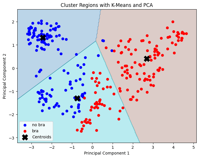
The graph illustrates the 2D projection of the data using Principal Component Analysis (PCA) alongside K-Means clustering, with points labeled based on their original categories: semi-nude women ("bra") and women wearing a shirt ("no bra"). The clustering regions defined by K-Means partially align with the labeled groups, as evidenced by distinct separations in some areas; however, overlapping regions indicate that the two principal components do not fully capture the variance required to separate the groups entirely. The centroids, marked as black crosses, provide a reference for the K-Means cluster centers, highlighting how the feature space is partitioned. These results suggest that while PCA provides some meaningful dimensionality reduction, additional components or more complex clustering methods may be necessary to achieve a clearer alignment between clusters and labels.

To assess the variation in cosine similarity between text-image pairs in the CLIP model after applying Sparse Autoencoders (SAEs), the differences were calculated by subtracting the original cosine similarity (without SAEs) from the results obtained with SAEs. For the 280 images analyzed, Factor x16 showed a mean difference of 3.75e-3 with a standard deviation of 3.94e-3, indicating moderate and consistent variation. Factor x32 exhibited the highest mean difference 4.15e-3 but also the largest variability 5.36e-3, suggesting it introduces the most significant changes. Conversely, Factor x8 had the lowest mean difference 3.46e-3 with moderate variability 4.52e-3, indicating minimal deviation from the original model. These results demonstrate that SAEs induce slight alterations in cosine similarity, with Factor x32 introducing the most notable changes at the expense of higher variability, while Factor x8 maintains closer alignment with the original CLIP model.

Metric	Difference $({\theta }_{Clip}-{\theta }_{ClipSAEX16})$	Difference $({\theta }_{Clip}-{\theta }_{ClipSAEX32})$	Difference $({\theta }_{Clip}-{\theta }_{ClipSAEX8})$
Mean	3.75e-3	4.15e-3	3.46e-3
Std	3.94e-3	5.36e-3	4.52e-3

 

5. Conclusion

Our implementation of Sparse Autoencoders (SAEs) using the Jumped SAE configuration on the CLIP Vision Transformer has demonstrated a robust methodology for decomposing and analyzing internal activations. Focusing on the technical aspects, we extracted the residual activations from layers 22, 23, and 24 of a curated dataset comprising 280 images, and we trained nine distinct SAE models with expansion factors of x8, x16, and x32 over 10,000 training steps.

Key implementation findings include:

• Training Dynamics and Metrics:
  By monitoring reconstruction loss, the L0 norm (indicating sparsity), and the Fraction of Variance Unexplained (FVU), we observed that lower expansion factors (e.g., x8) tend to yield lower reconstruction error while achieving less sparsity. In contrast, higher expansion factors (e.g., x32) enforce stricter sparsity but at the cost of increased reconstruction error and variability. Our systematic analysis identified that the configuration from Layer 22 with an expansion factor of x16 provided the best overall balance—achieving low reconstruction loss (3.65e-4), moderate sparsity (L0 = 5.62e-2), and acceptable FVU (1.43e-2).
• Latent Space Analysis:
  We conducted an in-depth evaluation of the learned latent representations by generating Sparsity vs. Fidelity graphs and computing average activation histograms across different image subsets. Logarithmic transformations improved the visibility of differences, allowing us to identify candidate neurons that exhibited class-specific activation patterns. Dimensionality reduction via Principal Component Analysis (PCA) combined with K-means clustering further revealed distinct groupings in the latent space, underscoring the efficacy of our SAE configurations in isolating meaningful features.
• Statistical Validation:
  Statistical tests—including the Kolmogorov-Smirnov Test, Mann–Whitney U Test, and calculations of effect size and Cliff’s Delta—were instrumental in quantifying differences between the activation distributions of the two image groups. These analyses confirmed that specific SAE configurations (notably Layer 22 with expansion factors x16 and x32) capture significant structural differences, thereby validating our selection of the optimal configuration for further analysis.
• Integration and Model Impact:
  Finally, by comparing the cosine similarity of the original CLIP model outputs with those produced after integrating the SAE processing, we observed only moderate variations. This indicates that while the SAE intervention induces slight shifts in the latent representations, it preserves the overall integrity of the CLIP model’s outputs.

In summary, our focused implementation and analysis of SAEs provides a detailed and reproducible framework for extracting interpretable features from deep vision models. The balance between reconstruction fidelity and sparsity—achieved through careful selection of model parameters—highlights the potential of this approach for further mechanistic interpretability studies and future applications that require precise control over latent representations.
 

0 comments

Comments sorted by top scores.