Are SAE features from the Base Model still meaningful to LLaVA?
post by Shan23Chen (shan-chen) · 2024-12-05T19:24:34.727Z · LW · GW · 2 commentsContents
  TL;DR:
  Introduction
    Some Background on LLaVA:
    Key Components
      Training:
    Evaluating SAE Transferability with LLaVA
  Experimental Design
    Dataset
    Features and Evaluation
  Is there any signal?
      1. Dolphin 🐬
      Layer 0
      Layer 6
      Layer 10
      Layer 12
      Layer 12-it
      2. Skyscraper 🏙️
      Layer 0
      Layer 6
      Layer 10
      Layer 12
      Layer 12-it
      3. Boy 👦
      Layer 0
      Layer 6
      Layer 10
      Layer 12
      Layer 12-it
      4. Cloud ☁️
      Layer 0
      Layer 6
      Layer 10
      Layer 12
      Layer 12-it
  Classification Analysis
    Classification Setup
      Layer Evaluation
  Classification Findings
    Performance Summary
      So, in a way, we actually nearly recovered the full VIT performance here!
    1. How Many Features Do We Need?
      2. Which Layer Performs Best?
      3. To Binarize or Not to Binarize?
      4. Data Efficiency: How Much Training Data Do We Need?
    Big Picture Insights
    What’s Next?
None
2 comments
Shan Chen, Jack Gallifant, Kuleen Sasse, Danielle Bitterman[1]
Please read this as a work in progress where we are colleagues sharing this in a lab (https://www.bittermanlab.org) meeting to help/motivate potential parallel research.
TL;DR:
- Recent work has evaluated the generalizability of Sparse Autoencoder (SAE) features; this study examines their effectiveness in multimodal settings.
- We evaluate feature extraction using a CIFAR-100-inspired explainable classification task, analyzing the impact of pooling strategies, binarization, and layer selection on performance.
- SAE features generalize effectively across multimodal domains and recover nearly 100% of the ViT performance (this LLaVA used).
- Feature extraction, particularly leveraging middle-layer features with binarized activations and larger feature sets, enables robust classification even in low-data scenarios, demonstrating the potential for simple models in resource-constrained environments.
Introduction
The pursuit of universal and interpretable features has long captivated researchers in AI, with Sparse Autoencoders (SAEs) emerging as a promising tool for extracting meaningful representations. Universality, in this context, refers to the ability of features to transcend domains, languages, modalities, model architectures, sizes, and training strategies. Recent advances have shed light on key properties of these representations, including their dataset-dependent nature, their relationship with the granularity of training data, and their transferability across tasks. Notably, studies have demonstrated the intriguing ability of features to transfer from base models to fine-tuned models, such as Kissane et al. (2024) [LW · GW] and Kutsyk et al. (2024) [AF · GW], and have even hinted at their generalization across layers (Ghilardi et al. 2024). However, one critical question remains underexplored: can features trained in unimodal contexts (e.g., text-only or image-only models) effectively generalize to multimodal systems?
In this work, we focus on bridging this "modality gap" by investigating the applicability of SAE-derived features in multimodal settings. Specifically, we explore LLaVA (Liu et al. 2024), a popular multimodal model that integrates vision and language tasks. Leveraging the CIFAR-100 dataset, which provides a challenging fine-grained classification task, we assess the transferability and interpretability of features learned from base models in this multimodal context. Through a detailed layer-wise analysis, we investigate the semantic evolution of tokens and evaluate the utility of these features in downstream classification tasks.
While previous work has largely focused on the unimodal-to-unimodal transfer of features, our experiments aim to answer whether features extracted from base models can effectively bridge the gap to multimodal applications. This exploration aligns with ongoing efforts to understand how features encode information, how transferable they are across different contexts, and how they can be interpreted when applied to diverse tasks.
This write-up details our exploratory experiments, including:
- Layer-wise Feature Analysis: Understanding how token-level representations evolve semantically across layers within the LLaVA framework.
- Classification Performance: Evaluating the utility of SAE-derived features on CIFAR-100 for fine-grained image classification.
- Transferability: Assessing the generalization of features trained in unimodal contexts to a multimodal setting.
Our findings contribute to advancing the interpretability and universality of features in large models, paving the way for more robust, explainable, and cross-modal AI systems.
Some Background on LLaVA:
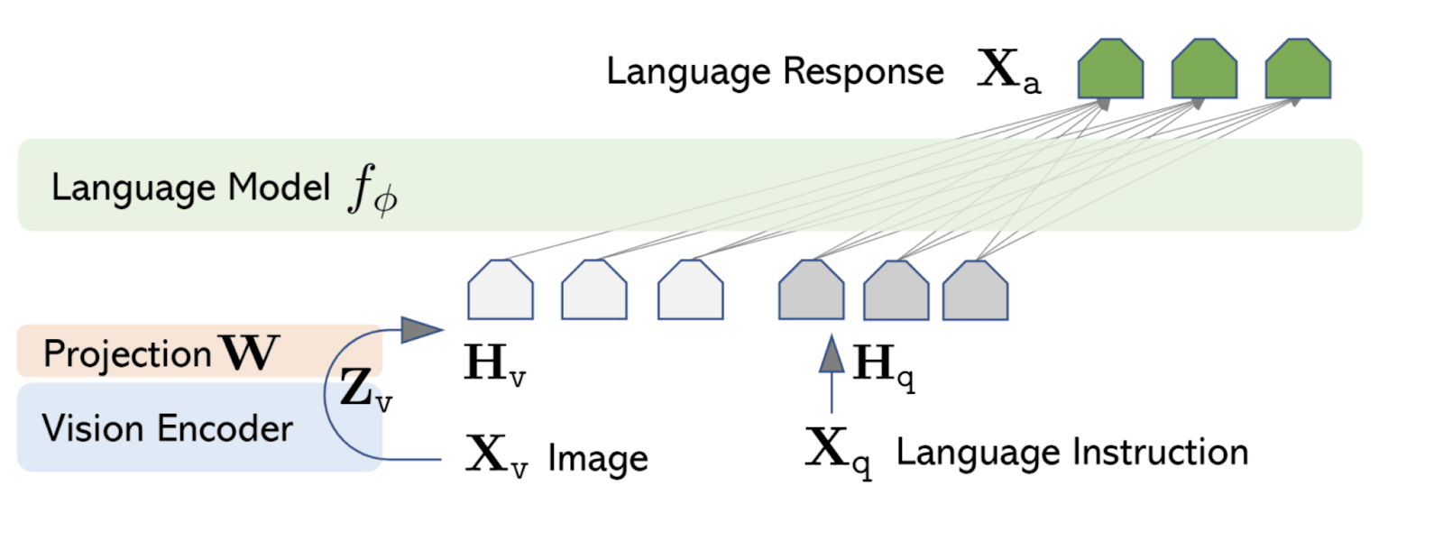
LLaVA (Liu et al. 2023) is a multimodal framework that integrates vision and language tasks. By combining a Vision Encoder and a Language Model, LLaVA processes both image and textual inputs to generate coherent and contextually appropriate language-based outputs.
Key Components
Vision Encoder:
- Image Processing: Utilizes a pre-trained CLIP ViT model to extract visual features from input images.
- Feature Projection: Transforms the extracted visual features through a projection layer to align them with the input space of the language model.
Language Model:
- Text Processing: Employs a pre-trained language model, Vicuna, to process textual inputs.
- Multimodal Integration: Combines the projected visual features with textual data to generate contextually relevant language outputs.
Token Structure:
- The model tokenizes the inputs into two tokens, including a Begin of Image (BoI) token and an End of Image (EoI) token, and each ViT patches into a text token;
- Image tokens and text tokens are processed together (aligning more towards the text space) for a unified understanding.
Output:
The final output of the LLaVA model is a text-based response that reflects both the visual content of the input image and the language instructions provided. This enables a wide range of applications, from answering questions about an image to generating detailed image captions.
Training:
LLaVA’s multimodal alignment is realized during visual instruction tuning, the fine-tuning of the Language Model using multimodal instruction-following data, where each textual instruction is paired with corresponding visual inputs. During this process, the model learns to interpret visual data in conjunction with textual context, which aligns visual features with language features.
Evaluating SAE Transferability with LLaVA
LLaVA’s architecture provides an ideal testbed for evaluating the transferability of SAEs. By leveraging its unified token space and multimodal alignment, we can assess how well unimodal features extracted by SAEs adapt to multimodal contexts. Specifically, LLaVA’s ability to process and integrate image and text tokens allows us to analyze the semantic evolution of SAE-derived features across its layers, offering insights into their utility and generalization capabilities in multimodal scenarios.
In this study, we utilize the Intel Gemma-2B LLaVA 1.5-based model (Intel/llava-gemma-2b) as the foundation for our experiments. For feature extraction, we incorporate pre-trained SAEs from jbloom/Gemma-2b-Residual-Stream-SAEs, trained on the Gemma-1-2B model. These SAEs include 16,384 features (an expansion factor of 8 × 2048) and are designed to capture sparse and interpretable representations.
Our analysis focuses on evaluating the layer-wise integration of these features within LLaVA to determine their effectiveness in bridging unimodal-to-multimodal gaps. Specifically, we assess their impact on semantic alignment, and classification performance. We hypothesized that the text-trained SAE features were still meaningful to LLaVA.
Experimental Design
Dataset
We used the CIFAR-100 (Krizhevsky et al. 2009) dataset, which comprises:
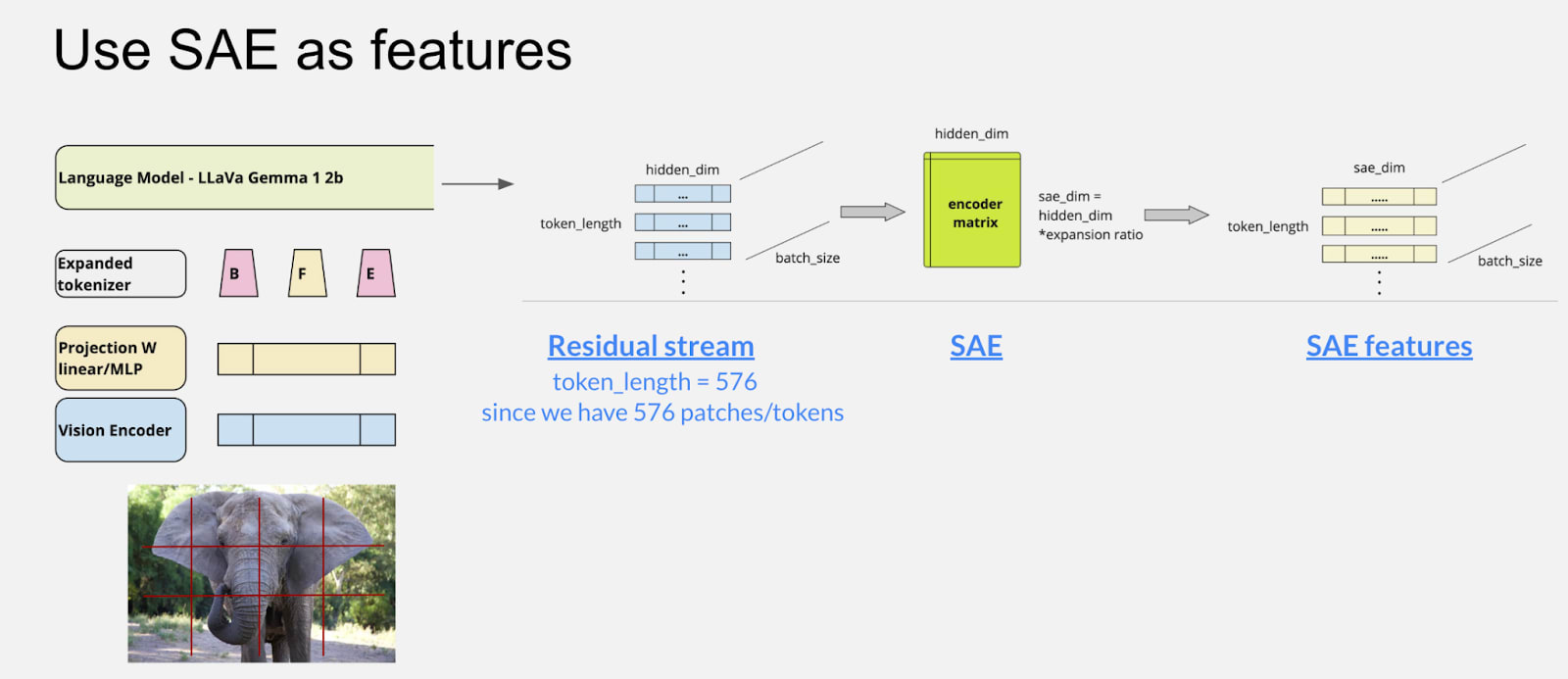
- Fine labels: Spanning 100 distinct categories (e.g., “elephant” as illustrated in Figure 1).
Features and Evaluation
- Feature representation: We extracted SAE embeddings consisting of 576 tokens derived from image patches.
- Linear Classifier: A linear probe using the End-of-Image (EoI) token.
- Evaluation Metric: The Macro F1 score to evaluate the balance between precision and recall across all classes.
- Layer-Wise Analysis: Feature dynamics were analyzed across layers (0, 6, 10, 12, and 12-it (using an instruct model trained SAE instead)).
Is there any signal?
We implemented the outlined procedure and analyzed the retrieved features to evaluate whether meaningful features could be identified through this transfer method. As a first step, a preliminary cleaning process was conducted to refine the feature set before delving into the detailed retrieved features and their auto-interpretability explanations.
The objective of the cleaning process was to eliminate features that appeared to be disproportionately represented across instances, which could introduce noise, diminish interpretability, or indicate unaligned or non-transferable features. Considering the CIFAR-100 dataset, which comprises 100 labels with 100 instances per label, the expected maximum occurrence of any feature under uniform distribution is approximately 100. To address potential anomalies, a higher threshold of 1000 occurrences was selected as the cutoff for identifying and excluding overrepresented features. This conservative threshold ensured that dominant, potentially less informative features were removed while retaining those likely to contribute meaningfully to the analysis.
After cleaning, we examined the retrieved features across different model layers (0–12 of 19 layers). A clear trend emerged: deeper layers exhibited increasingly useful features.
Below, we provide examples of retrieved features from both high-performing and underperforming classes, demonstrating the range of interpretability outcomes:
1. Dolphin 🐬
Layer 0
- Top 2 Features shared across 100 instances:
- 16k/12746 (30/100 occurrences): Technical information related to cooking recipes and server deployment
- 16k/4154 (26/100 occurrences): References to international topics or content
Layer 6
- Top 2 Features shared across 100 instances:
- 16k/4090 (25/100 occurrences): Phrases related to a specific book title: The Blue Zones
- 16k/9019 (17/100 occurrences): Mentions of water-related activities and resources in a community context
Layer 10
- Top 2 Features shared across 100 instances:
- 16k/14117 (88/100 occurrences): Terms related to underwater animals and marine research
- 16k/6592 (61/100 occurrences): Actions involving immersion, dipping, or submerging in water
Layer 12
- Top 2 Features shared across 100 instances:
- 16k/6878 (77/100 occurrences): Terms related to oceanic fauna and their habitats
- 16k/13022 (53/100 occurrences): References to the ocean
Layer 12-it
- Top 2 Features shared across 100 instances:
- 16k/9486 (60/100 occurrences): Mentions of the ocean
- 16k/14295 (40/100 occurrences): Terms related to maritime activities, such as ships, sea, and naval battles
2. Skyscraper 🏙️
Layer 0
- Top 2 Features shared across 100 instances:
- 16k/12608 (11/100 occurrences): Information related to real estate listings and office spaces
- 16k/980 (7/100 occurrences): References to sports teams and community organizations
Layer 6
- Top 2 Features shared across 100 instances:
- 16k/1840 (32/100 occurrences): Details related to magnification and inspection, especially for physical objects and images
- 16k/12016 (28/100 occurrences): Especially for physical objects and images
Layer 10
- Top 2 Features shared across 100 instances:
- 16k/12480 (68/100 occurrences): References to physical structures or buildings
- 16k/1658 (62/100 occurrences): Character names and references to narrative elements in storytelling
Layer 12
- Top 2 Features shared across 100 instances:
- 16k/8373 (87/100 occurrences): References to buildings and structures
- 16k/6367 (61/100 occurrences): Locations and facilities related to sports and recreation
Layer 12-it
- Top 2 Features shared across 100 instances:
- 16k/7926 (78/100 occurrences): Terms related to architecture and specific buildings
- 16k/8783 (57/100 occurrences): References to the sun
3. Boy 👦
Layer 0
- Top 2 Features shared across 100 instances:
- 16k/980 (17/100): References to sports teams and community organizations
- 16k/4181 (10/100): Words related to communication and sharing of information
Layer 6
- Top 2 Featuresd share across 100 instances:
- 16k/14957 (52/100): Phrases related to interior design elements, specifically focusing on color and furnishings
- 16k/11054 (25/100): Hair styling instructions and descriptions
Layer 10
- Top 2 Features shared across 100 instances:
- 16k/4896 (87/100): Descriptions of attire related to cultural or traditional clothing
- 16k/11882 (83/100): References to familial relationships, particularly focusing on children and parenting
Layer 12
- Top 2 Features shared across 100 instances:
- 16k/5874 (89/100): Words associated with clothing and apparel products
- 16k/11781 (60/100): Phrases related to parental guidance and involvement
Layer 12-it
- Top 2 Features shared across 100 instances:
- 16k/6643 (88/100): Patterns related to monitoring and parental care
- 16k/9663 (67/100): Descriptions related to political issues and personal beliefs[2]
4. Cloud ☁️
Layer 0
- Top 2 Features shared across 100 instances:
- 16k/8212 (4/100): Possessive pronouns referring to one's own or someone else's belongings or relationships
- 16k/980 (3/100): References to sports teams and community organizations
Layer 6
- Top 2 Features shared across 100 instances:
- 16k/11048 (24/100): Descriptive words related to weather conditions
- 16k/2044 (21/100): Mentions of astronomical events and celestial bodies
Layer 10
- Top 2 Features shared across 100 instances:
- 16k/15699 (62/100): Terms related to aerial activities and operations
- 16k/1301 (59/100): References and descriptions of skin aging or skin conditions
Layer 12
- Top 2 Features shared across 100 instances:
- 16k/7867 (92/100): Themes related to divine creation and celestial glory
- 16k/7414 (89/100): Terms related to cloud computing and infrastructure
Layer 12-it
- Top 2 Features shared across 100 instances:
- 16k/11234 (80/100): The word "cloud" in various contexts
- 16k/8783 (47/100): References to the sun
Classification Analysis
Building on the feature extraction process, we shifted focus to an equally critical question: Could the extracted features meaningfully classify CIFAR-100 labels? Specifically, we aimed to determine whether these features could reliably distinguish between diverse categories such as "dolphin" and "skyscraper." Additionally, we investigated how choices like binarization and layer selection influenced the robustness and effectiveness of the classification process.
Here, we outline our methodology, key findings, and their broader implications.
Classification Setup
We implemented a linear classification pipeline to evaluate the retrieved features' predictive utility. Features were collected from multiple layers of the model and underwent the following preparation steps:
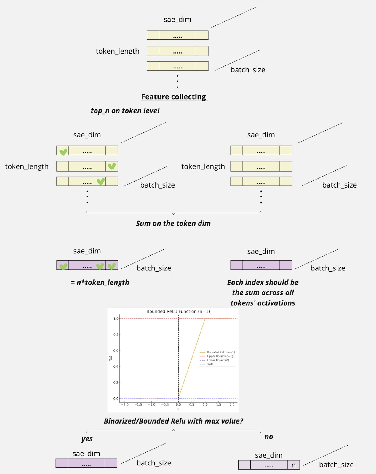
Feature Pooling:
Features were aggregated along the token dimension using two strategies:
- Summation: Calculated the sum of activations across tokens.
- Top-N Selection: Selected the highest N activations, representing the most salient features.
Activation Transformation:
We explored the impact of activation scaling on performance:
- Binarized Activations: Applied bounding to cap feature values, enforcing a more discrete representation of just showing whether this feature is activated or not.
- Non-Binarized Activations: Retained the original, unbounded feature values to preserve granularity.
Layer Evaluation
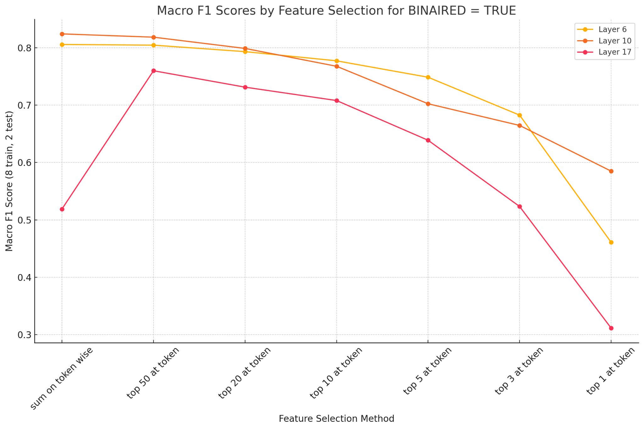
Features were extracted from Layers 6, 10, and 17 of the model. A linear classifier was trained using the features of each layer, and performance was assessed with Macro F1 scores. This ensured a balanced evaluation across all CIFAR-100 categories, allowing us to identify robustness, efficiency, and interpretability trends across different configurations.
Classification Findings
Performance Summary
- So, here are several baselines[3] (0.83 from LLaVa):
- Using EoI(End of Image) tokens, the linear probe achieved a Macro F1 score of 0.48
- Resnet has a Macro F1 of 0.75
- The same VIT in the model has a Macro F1 of 0.85
So, in a way, we actually nearly recovered the full VIT performance here!
- Results demonstrated high efficiency even with limited training data, validating the transferability of SAE embeddings.
1. How Many Features Do We Need?
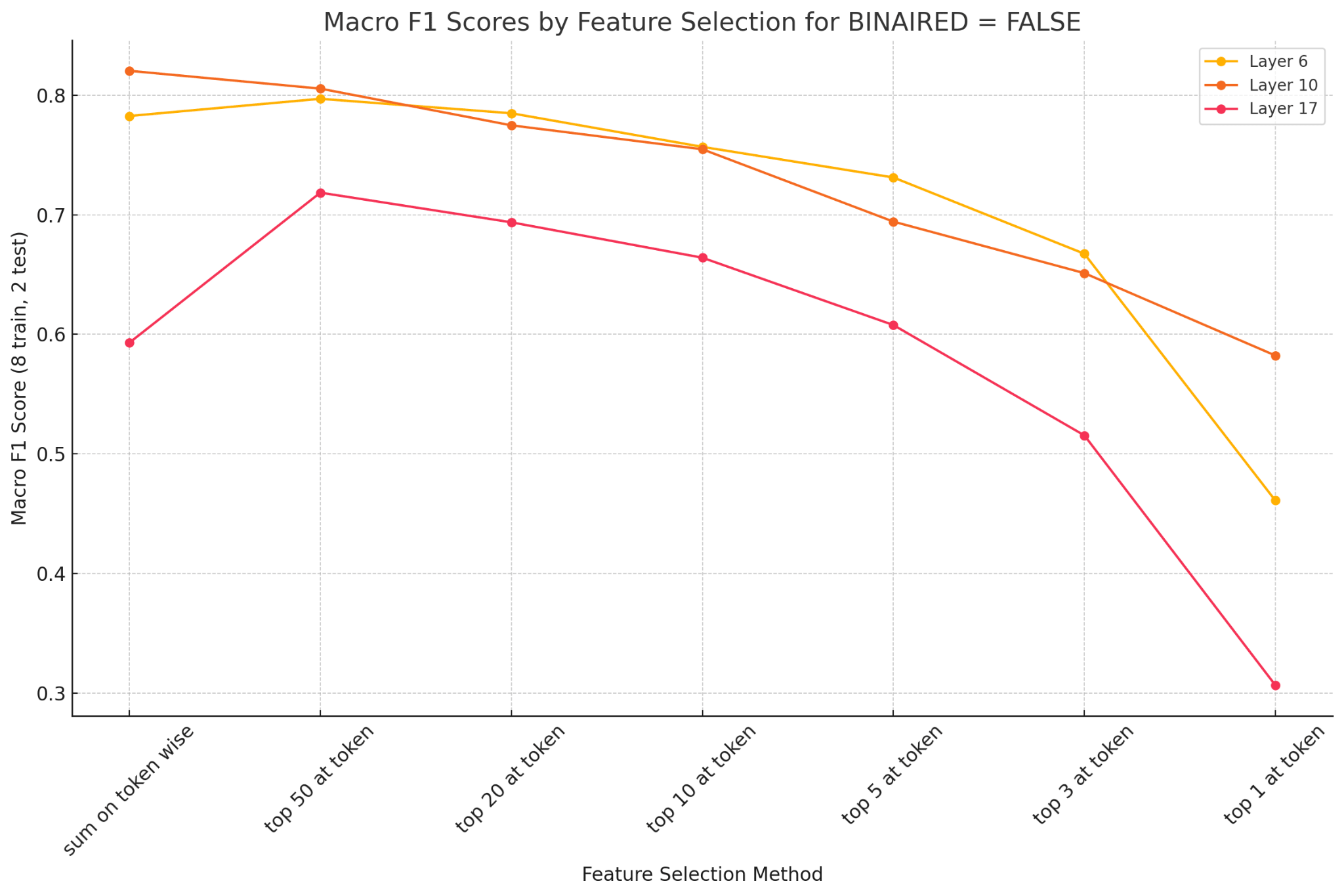
We tested a range of feature selection methods, from summing activations over all tokens to taking only the top-1 activation per token.
What We Found:
- Effect of Feature Selection: Summing activations across tokens or selecting top-50 activations consistently outperformed more restrictive methods (e.g., top-10, top-5 or top-3).
- Performance Trends: Excessive feature reduction led to performance degradation, with notable drops observed below the top-10 threshold.
Takeaway: Retaining a larger set of features preserves more discriminative information for CIFAR100, and this may have different imports across layers).
2. Which Layer Performs Best?
We tested features from Layers 6, 10, and 17 to see which part of the model provided the best representations.
What We Found:
Layer 10 Superiority: Features from Layer 10 consistently achieved the highest Macro F1 scores, balancing generalization and specificity.
- Layer 6 and 17 Performance: Layer 6 performed moderately well but required larger feature sets. Layer 17 showed reduced performance, likely due to its task-specific overspecialization.
Takeaway: Mid-level features (Layer 10) offered the best trade-off for CIFAR-100 classification.
3. To Binarize or Not to Binarize?
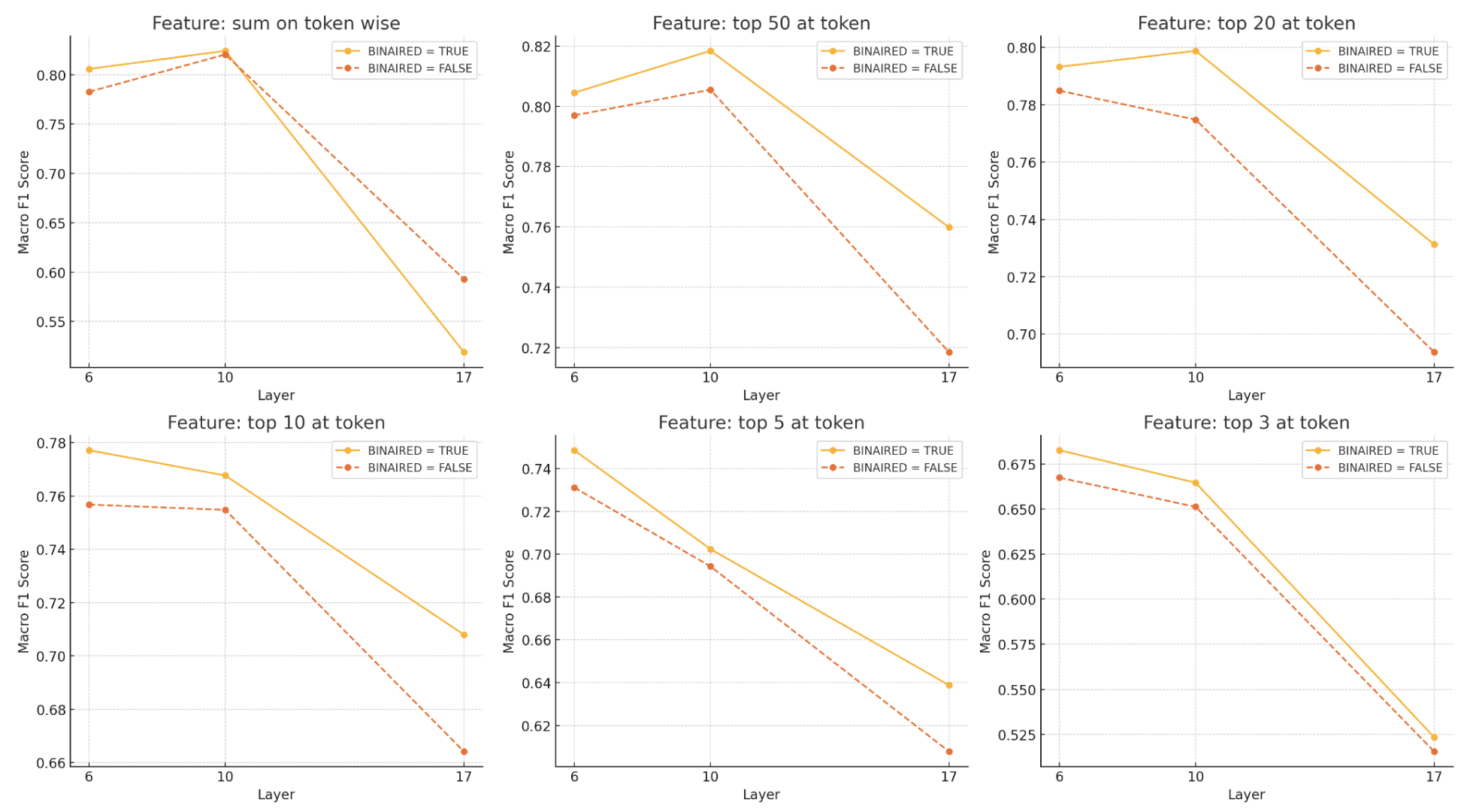
We compared binarized activations, which have cap values, with non-binarized ones. The idea is that binarization reduces noise and keeps things simple.
What We Found:
Binarized vs. Non-Binarized: Binarized features outperformed non-binarized counterparts, particularly with smaller feature sets.
- Impact by Feature Budget: The advantage of binarization was most evident in scenarios with fewer selected features (e.g., top-3 or top-5).
Takeaway: Binarization improves performance, especially under limited feature budgets.
4. Data Efficiency: How Much Training Data Do We Need?
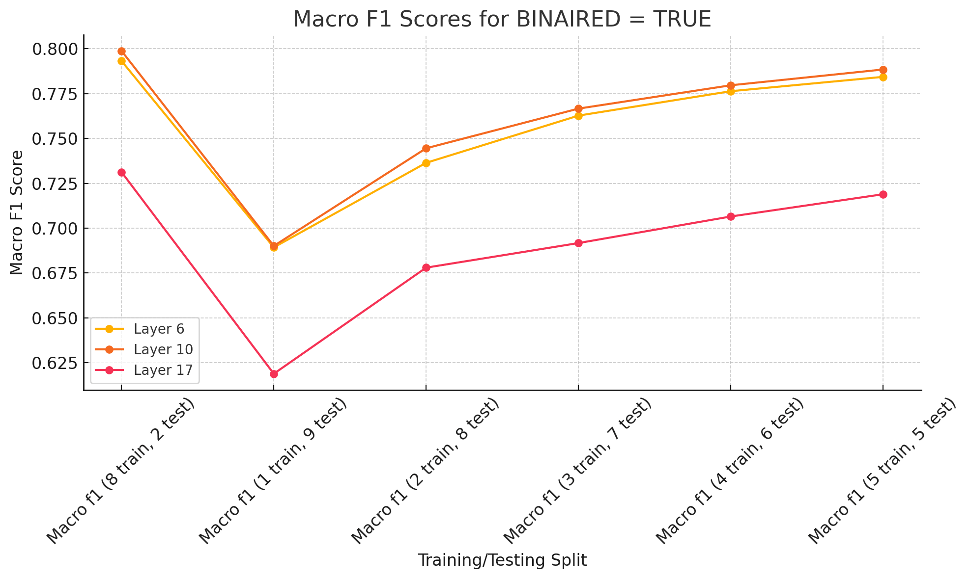
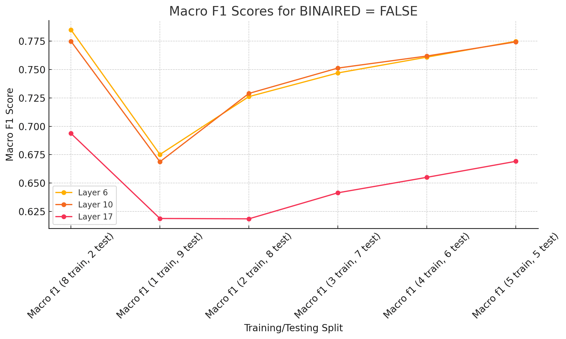
We tested how well the features worked when we varied the amount of training data, from small splits (1 train, 9 test) to larger splits (5 train, 5 test).
What We Found:
- Performance with Reduced Data: Binarized features from Layers 6 and 10 performed reliably with minimal training data (e.g., 1 train, 9 test split).
Layer 17 Limitations: Performance for Layer 17 improved with increased data but lagged under low-data conditions.
Takeaway: Binarized middle-layer features (e.g., Layer 10) were the most data-efficient option.
Big Picture Insights
So, what did we learn from all this? Here are the three big takeaways:
- More Features = Better Results: Don’t be stingy with feature selection. Larger feature sets lead to better classification, especially with middle layers.
- Binarization is a Game-Changer: It’s simple but effective. By capping activations, binarization reduces noise and makes features more robust, particularly in low-resource scenarios.
- Layer Choice Matters: Not all layers are created equal. Middle layers (like Layer 10) provided the best representations, balancing generalization and specificity.
What’s Next?
These findings open up exciting transfer learning and feature design possibilities in multimodal systems. We’ve shown that thoughtful feature selection and transformation can make a big difference even with simple linear classifiers.
For future work, we’re interested in exploring:
- Multimodal Extension: Expanding this methodology to other modalities, such as text or audio, to evaluate how feature transferability differs across domains.
- Enhanced Interpretability: Developing more precise methods to explain why certain layers or transformations (e.g., binarization) produce superior features. This could involve deeper mechanistic studies or visualization techniques.
- Layer Fusion Strategies
Exploring whether combining features from multiple layers offers additional performance gains. Could a hybrid approach outperform the best single-layer features?
- ^
The authors acknowledge financial support from the Google PhD Fellowship (SC), the Woods Foundation (DB, SC, JG), the NIH (NIH R01CA294033 (SC, JG, DB), NIH U54CA274516-01A1 (SC, DB) and the American Cancer Society and American Society for Radiation Oncology, ASTRO-CSDG-24-1244514-01-CTPS Grant DOI #: https://doi.org/10.53354/ACS.ASTRO-CSDG-24-1244514-01-CTPS.pc.gr.222210 (DB)
- ^
It is very intersting that models are more focusing on the cloth and potential parental care here.
Which lead me to think another question here, should we train SAE jointly for vision and text, or should we do it separately for multimodal systems.
- ^
We actually did image_net 1k too, and it is still running due to size. We are seeing 0.49 Macro F1 for layer 6...
2 comments
Comments sorted by top scores.
comment by houjing wei (houjing-wei) · 2025-02-06T17:25:47.868Z · LW(p) · GW(p)
Thank you very much for this highly insightful blog! I am a beginner in SAE but am very interested in how SAE can be used to interpret modern LLM-based vision-language models.
May I ask if the experiments in your blog have code available for sharing?
Replies from: shan-chen↑ comment by Shan23Chen (shan-chen) · 2025-02-12T18:15:08.539Z · LW(p) · GW(p)
thank you! full paper and code will be ready soon!