Progress on Causal Influence Diagrams

post by tom4everitt · 2021-06-30T15:34:33.381Z · LW · GW · 6 comments

Contents

  What are causal influence diagrams?
  Incentive Concepts
  User Interventions and Interruption
  Reward Tampering
  Multi-Agent CIDs
  Software
  Looking ahead
  List of recent papers:
None
6 comments

By Tom Everitt, Ryan Carey, Lewis Hammond, James Fox, Eric Langlois, and Shane Legg

Crossposted from DeepMind Safety Research

About 2 years ago, we released the first few papers on understanding agent incentives using causal influence diagrams. This blog post will summarize progress made since then.

What are causal influence diagrams?

A key problem in AI alignment is understanding agent incentives. Concerns have been raised that agents may be incentivized to avoid correction, manipulate users, or inappropriately influence their learning. This is particularly worrying as training schemes often shape incentives in subtle and surprising ways. For these reasons, we’re developing a formal theory of incentives based on causal influence diagrams (CIDs).

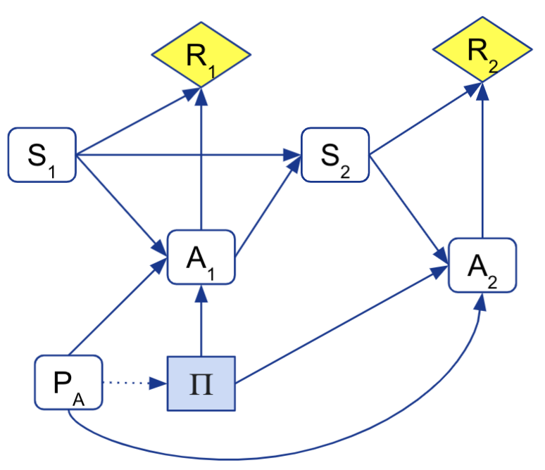
Here is an example of a CID for a one-step Markov decision process (MDP). The random variable S₁ represents the state at time 1, A₁ represents the agent’s action, S₂ the state at time 2, and R₂ the agent’s reward. 

The action A₁ is modeled with a decision node (square) and the reward R₂ is modeled as a utility node (diamond), while the states are normal chance nodes (rounded edges). Causal links specify that S₁ and A₁ influence S₂, and that S₂ determines R₂. The information link S₁ → A₁ specifies that the agent knows the initial state S₁ when choosing its action A₁.

In general, random variables can be chosen to represent agent decision points, objectives, and other relevant aspects of the environment.

In short, a CID specifies:

• Agent decisions
• Agent objectives
• Causal relationships in the environment
• Agent information constraints

These pieces of information are often essential when trying to figure out an agent’s incentives: how an objective can be achieved depends on how it is causally related to other (influenceable) aspects in the environment, and an agent’s optimization is constrained by what information it has access to. In many cases, the qualitative judgements expressed by a (non-parameterized) CID suffice to infer important aspects of incentives, with minimal assumptions about implementation details. Conversely, it has been shown that it is necessary to know the causal relationships in the environment to infer incentives, so it’s often impossible to infer incentives with less information than is expressed by a CID. This makes CIDs natural representations for many types of incentive analysis.

Other advantages of CIDs is that they build on well-researched topics like causality and influence diagrams, and so allows us to leverage the deep thinking that’s already been done in these fields.

Incentive Concepts

Having a unified language for objectives and training setups enables us to develop generally applicable concepts and results. We define four such concepts in Agent Incentives: A Causal Perspective (AAAI-21):

• Value of information: what does the agent want to know before making a decision?
• Response incentive: what changes in the environment do optimal agents respond to?
• Value of control: what does the agent want to control?
• Instrumental control incentive: what is the agent both interested and able to control?

For example, in the one-step MDP above:

• For S_1, an optimal agent would act differently (i.e. respond) if S₁ changed, and would value knowing and controlling S₁, but it cannot influence S₁ with its action. So S₁ has value of information, response incentive, and value of control, but not an instrumental control incentive.
• For S₂ and R₂, an optimal agent could not respond to changes, nor know them before choosing its action, so these have neither value of information nor a response incentive. But the agent would value controlling them, and is able to influence them, so S₂ and R₂ have value of control and instrumental control incentive.

In the paper, we prove sound and complete graphical criteria for each of them, so that they can be recognized directly from a graphical CID representation (see previous blog posts).

Value of information and value of control are classical concepts that have been around for a long time (we contribute to the graphical criteria), while response incentives and instrumental control incentives are new concepts that we have found useful in several applications.

For readers familiar with previous iterations of this paper, we note that some of the terms have been updated. Instrumental control incentives were previously called just “control incentives”. The new name emphasizes that it’s control as an instrumental goal, as opposed to control arising as a side effect (or due to mutual information [AF · GW]). Value of information and value of control were previously called “observation incentives” and “intervention incentives”, respectively.

User Interventions and Interruption

Let us next turn to some recent applications of these concepts. In How RL Agents Behave when their Actions are Modified (AAAI-21), we study how different RL algorithms react to user interventions such as interruptions and over-ridden actions. For example, Saunders et al. developed a method for safe exploration where a user overrides dangerous actions. Alternatively, agents might get interrupted if analysis of their “thoughts” (or internal activations) suggest they are planning something dangerous. How do such interventions affect the incentives of various RL algorithms?

First, we formalize action-modification by extending MDPs with a parameter P_A that describes action-modification. We then model such modified-action MDPs with a CID: 

Here we model the agent’s policy Π as the decision rather than the actions A_i, as the latter are not under full control of the agent, but can also be influenced by the action-modification P_A (as represented by arrows P_A → A_i and Π → A_i). The agent might know the interruption scheme P_A from interruptions during training, so we include an information link P_A → Π.

We analyze different prototypical RL algorithms in terms of the causal assumptions they make on the environment:

• Black-box optimization algorithms such as evolutionary strategies take into account all causal relationships.
• In contrast, the update rule of Q-learning effectively assumes that the next action will be taken optimally, with no action-modification. This means that Q-learners ignore causal effects P_A -> A. Similarly, SARSA with the action chosen by the agent in the TD-update assumes that it will be in control of its next action. We call this version virtual SARSA.
• SARSA based on the modified action (empirical SARSA) ignores the effect of action-modification on the current action, but takes into account the effect on subsequent actions.

We can represent the differences with the following CIDs. (The extra policy node Π’ for empirical SARSA represents that action are optimized separately rather than jointly.) 

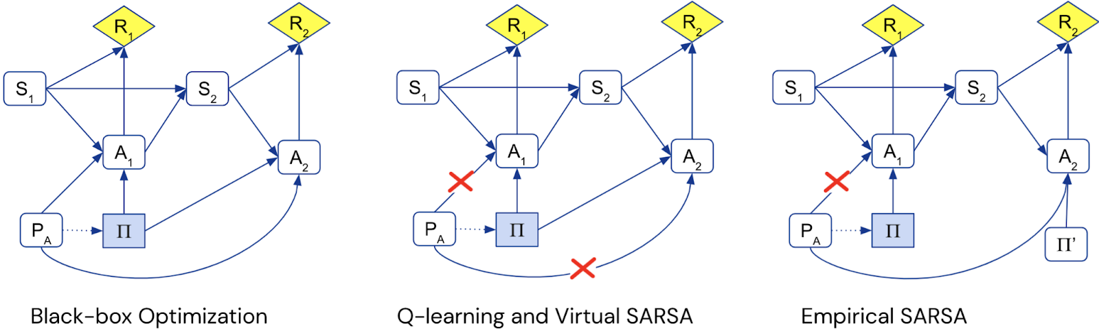
The CIDs can be used to understand how the different algorithms adapt to interruption, via a graphical criterion for path-specific response incentives. Black-box optimization tries to both obscure its policy and to disable its off-switch, whereas Q-learning and Virtual SARSA do neither. Empirical SARSA tries to disable the off-switch, but does not try to obscure its policy. 

We verify these results empirically in the relevant AI safety gridworlds, as well as in one new environment where the agent has to behave well in simulation to be deployed in reality, where black-box optimizers exhibit “treacherous turn [LW · GW]”-like behavior. The results are a generalization of Orseau and Armstrong’s interruptibility results for Q-learning and SARSA.

Zooming out, these results are a good example of causal analysis of ML algorithms. Different design choices translate into different causal assumptions, which in turn determine the incentives. In particular, the analysis highlights why the different incentives arise, thus deepening our understanding of how behavior is shaped.

Reward Tampering

Another AI safety problem that we have studied with CIDs is reward tampering. Reward tampering can take several different forms, including the agent:

• rewriting the source code of its implemented reward function (“wireheading”),
• influencing users that train a learned reward model (“feedback tampering”),
• manipulating the inputs that the reward function uses to infer the state (“RF-input tampering / delusion box problems”).

For example, the problem of an agent influencing its reward function may be modeled with the following CID, where RFᵢ represent the agent’s reward function at different time steps, and the red links represent an undesirable instrumental control incentive.

In Reward Tampering Problems and Solutions (published in the well-respected philosophy journal Synthese) we model all these different problems with CIDs, as well as a range of  proposed solutions such as current-RF optimization, uninfluenceable reward learning, and model-based utility functions. Interestingly, even though these solutions were initially developed independently of formal causal analysis, they all avoid undesirable incentives by cutting some causal links in a way that avoids instrumental control incentives. 

By representing these solutions in a causal framework, we can get a better sense of why they work, what assumptions they require, and how they relate to each other. For example, current-RF optimization and model-based utility functions both formulate a modified objective in terms of an observed random variable from a previous time step, whereas uninfluenceable reward learning (such as CIRL) uses a latent variable:

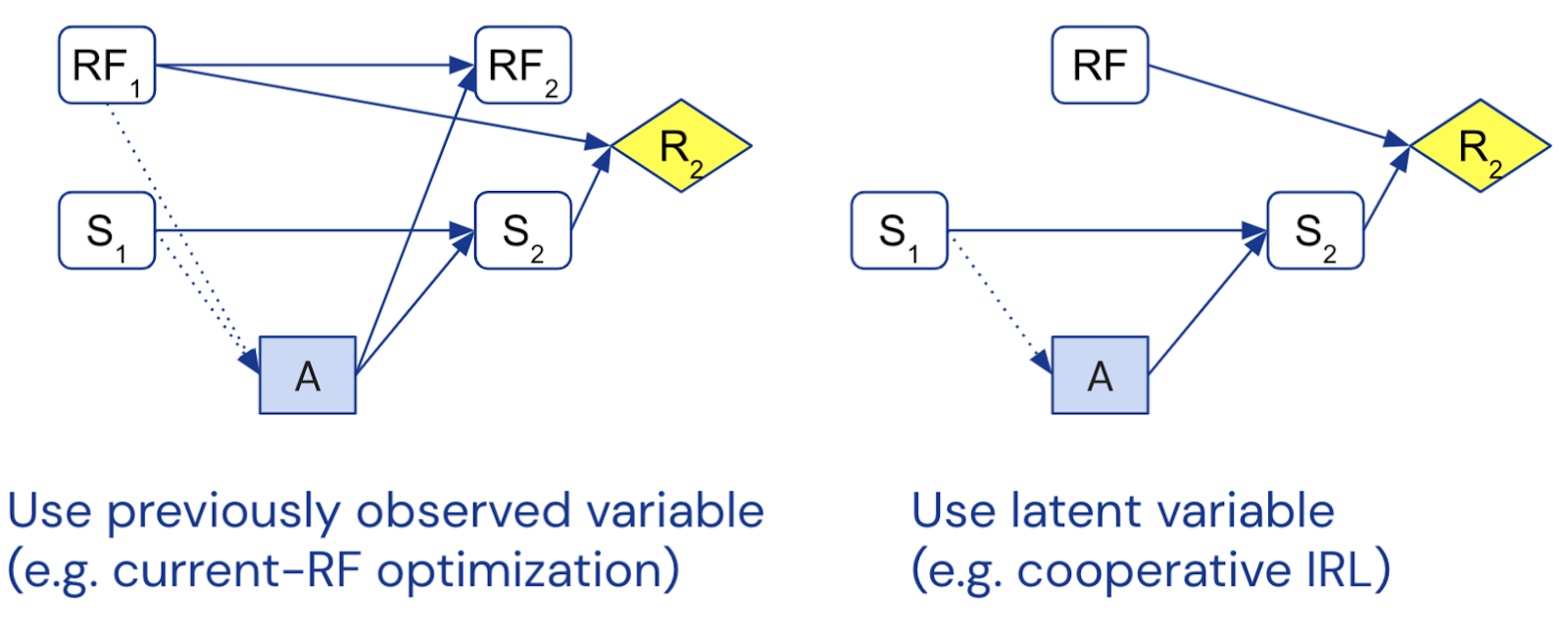
As a consequence, the former methods must deal with time-inconsistency and a lack of incentive to learn, while the latter requires inference of a latent variable. It will likely depend on the context whether one is preferable over the other, or if a combination is better than either alone. Regardless, having distilled the key ideas should put us in a better position to flexibly apply the insights in novel settings.

We refer to the previous blog post for a longer summary of current-RF optimization. The paper itself has been significantly updated since previously shared preprints.

Multi-Agent CIDs

Many interesting incentive problems arise when multiple agents interact, each trying to optimize their own reward while they simultaneously influence each other's payoff. In Equilibrium Refinements in Multi-Agent Influence Diagrams (AAMAS-21), we begin to lay some foundations for understanding multi-agent situations with multi-agent CIDs (MACIDs). 

First, we relate MACIDs to extensive-form games (EFGs), currently the most popular graphical representations of games. While EFGs sometimes offer more natural representations of games, they have some significant drawbacks compared to MACIDs. In particular, EFGs can be exponentially larger, don’t represent conditional independencies, and lack random variables to apply incentive analysis to.

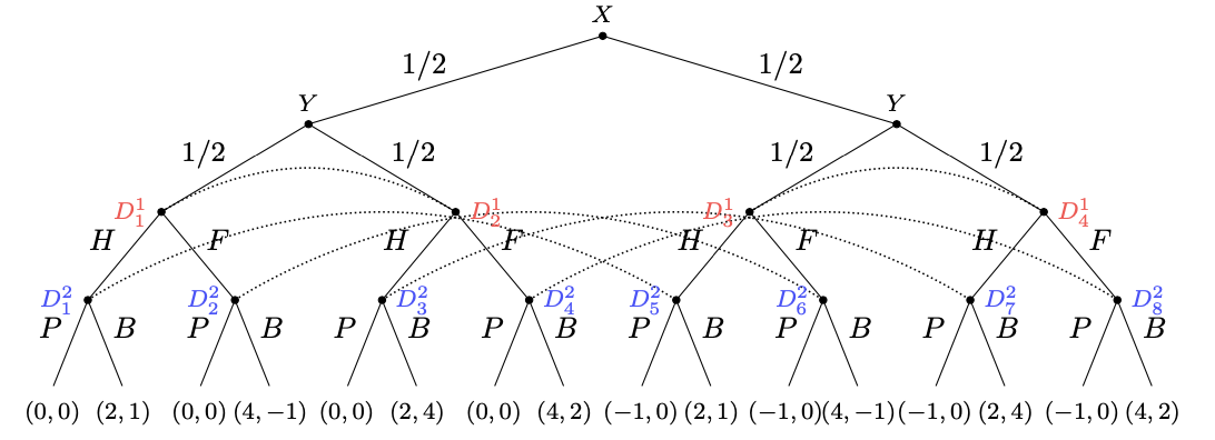
As an example, consider a game where a store (Agent 1) decides (D¹) whether to charge full (F) or half (H) price for a product depending on their current stock levels (X), and a customer (Agent 2) decides (D²) whether to buy it (B) or pass (P) depending on the price and how much they want it (Y). The store tries to maximize their profit U¹, which is greater if the customer buys at a high price. If they are overstocked and the customer doesn’t buy, then they have to pay extra rent. The customer is always happy to buy at half price, and sometimes at full price (depending on how much they want the product).

The EFG representation of this game is quite large, and uses information sets (represented with dotted arcs) to represent the facts that the store doesn’t know how much the customer wants the gadget, and that the customer doesn’t know the store’s current stock levels:

In contrast, the MACID representation is significantly smaller and clearer. Rather than relying on information sets, the MACID uses information links (dotted edges) to represent the limited information available to each player:

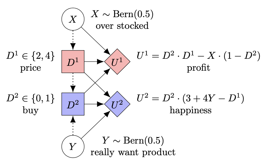
Another aspect that is made more clear from the MACID, is that for any fixed customer decision, the store’s payoff is independent of how much the customer wanted the product (there’s no edge Y→U¹). Similarly, for any fixed product price, the customer’s payoff is independent of the store’s stock levels (no edge X→U²). In the EFG, these independencies could only be inferred by looking carefully at the payoffs.

One benefit of MACIDs explicitly representing these conditional independencies is that more parts of the game can be identified as independently solvable. For example, in the MACID, the following independently solvable component can be identified. We call such components MACID subgames:

Solving this subgame for any value of D¹ reveals that the customer always buys when they really want the product, regardless of whether there is a discount. This knowledge makes it simpler to next compute the optimal strategy for the store. In contrast, in the EFG the information sets prevent any proper subgames from being identified. Therefore, solving games using a MACID representation is often faster than using an EFG representation.

Finally, we relate various forms of equilibrium concepts between MACIDs and EFGs. The most famous type of equilibrium is the Nash equilibrium, which occurs when no player can unilaterally improve their payoff. An important refinement of the Nash equilibrium is the subgame perfect equilibrium, which rules out non-credible threats by requiring that a Nash equilibrium is played in every subgame. An example of a non-credible threat in the store-customer game would be the customer “threatening” the store to only buy at a discount. The threat is non-credible, since the best move for the customer is to buy the product even at full price, if he really wants it. Interestingly, only the MACID version of subgame perfectness is able rule such threats out, because only in the MACID is the customer’s choice recognized as a proper subgame. 

Ultimately, we aim to use MACIDs to analyze incentives in multi-agent settings. With the above observations, we have put ourselves in position to develop a theory of multi-agent incentives that is properly connected to the broader game theory literature.

Software

To help us with our research on CIDs and incentives, we’ve developed a Python library called  PyCID, which offers:

• A convenient syntax for defining CIDs and MACIDs,
• Methods for computing optimal policies, Nash equilibria, d-separation, interventions, probability queries, incentive concepts, graphical criteria, and more,
• Random generation of (MA)CIDs, and pre-defined examples.

No setup is necessary, as the tutorial notebooks can be run and extended directly in the browser, thanks to Colab.

We’ve also made available a Latex package for drawing CIDs, and have launched causalincentives.com as a place to collect links to the various papers and software that we’re producing.

Looking ahead

Ultimately, we hope to contribute to a more careful understanding of how design, training, and interaction shapes an agent’s behavior. We hope that a precise and broadly applicable language based on CIDs will enable clearer reasoning and communication on these issues, and facilitate a cumulative understanding of how to think about and design powerful AI systems.

From this perspective, we find it encouraging that several other research groups have adopted CIDs to:

• Analyze the incentives of unambitious agents to break out of their box,
• Explain uninfluenceable reward learning, and clarifying its desirable properties (see also Section 3.3 in the reward tampering paper),
• Develop a novel framework to make agents indifferent to human interventions.

We’re currently to pursuing several directions of further research:

• Extending the general incentive concepts to multiple decisions and multiple agents.
• Applying them to fairness and other AGI safety settings.
• Analysing limitations that have been identified with work so far. Firstly, considering the issues raised by Armstrong and Gorman. And secondly, [AF · GW] looking at broader concepts than instrumental control incentives, as influence can also be incentivized as a side-effect of an objective.
• Probing further at their philosophical foundations, and establishing a clearer semantics for decision and utility nodes.

Hopefully we’ll have more news to share soon.

Thanks for reading, and please comment and/or get in touch in other ways if you have any thoughts!

We would like to thank Neel Nanda, Zac Kenton, Sebastian Farquhar, Carolyn Ashurst, and Ramana Kumar for helpful comments on drafts of this post.

List of recent papers:

• Agent Incentives: A Causal Perspective
• How RL Agents Behave When Their Actions Are Modified
• Reward tampering problems and solutions in reinforcement learning: A causal influence diagram perspective
• Equilibrium Refinements for Multi-Agent Influence Diagrams: Theory and Practice

See also causalincentives.com

6 comments

Comments sorted by top scores.