Language Models Use Trigonometry to Do Addition

post by Subhash Kantamneni (subhashk) · 2025-02-05T13:50:08.243Z · LW · GW · 0 comments

Contents

  TLDR 
  Motivation and Problem Setting
  LLMs Represent Numbers on a Helix
    Investigating the Structure of Numbers
      Periodicity
      Linearity
    Parameterizing Numbers as a Helix
    Fitting a Helix
    Evaluating the Helical Fit
    Relation to the Linear Representation Hypothesis[2] 
    Is the helix the full story?
  LLMs Use the Clock Algorithm to Compute Addition 
    Understanding MLPs
    Zooming in on Neurons
      Modeling Neuron Preactivations
      Understanding MLP Inputs
    Interpreting Model Errors
  Limitations
  Conclusion
None
No comments

I (Subhash) am a Masters student in the Tegmark AI Safety Lab at MIT.  I am interested in recruiting for full time roles this Spring - please reach out if you're interested in working together!

TLDR 

This blog post accompanies the paper "Language Models Use Trigonometry to Do Addition." Key findings:

• We show that LLMs represent numbers on a helix
  • This helix has circular features (sines and cosines) with periods $T=[2,5,10,100]$ and a linear component
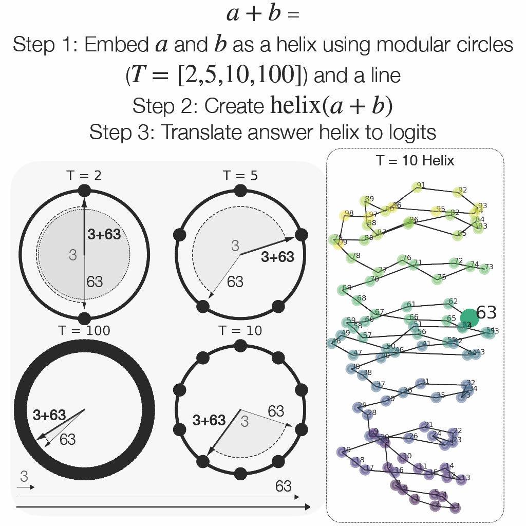
• To solve $a+b$, we claim that LLMs manipulate the helix for $a$ and $b$ to create the helix for $a+b$ using a form of the Clock algorithm introduced by Nanda, et al.
  • This is conceptually akin to going from $\cos \left(a\right),\cos \left(b\right)$ to $\cos (a+b)$
  • Intuitively, it's like adding angles on a Clock face.

Motivation and Problem Setting

Mathematical reasoning is an increasingly prominent measure of LLM capabilities, yet we lack understanding of how LLMs process even simple mathematical tasks. In this spirit, we aim to reverse engineer how three mid-sized LLMs compute addition.

In this blog post, we focus on GPT-J, a 6B parameter LLM, but we show additional results for Pythia-6.9B and Llama3.1-8B in the main paper. We construct problems of the form  $a+b$ for $a,b\in [0,99]$. GPT-J is competent on this task, successfully completing 80% of prompts. 

For conciseness, we share a subset of our results here. Please see the full paper for additional information.

LLMs Represent Numbers on a Helix

Investigating the Structure of Numbers

To generate a ground up understanding of how LLMs compute $a+b$, we first aim to understand how they represent some integer $a$. In order to identify trends in their representation, we run GPT-J on all single-token integers $a\in [0,360]$. We conduct analysis on the residual stream following layer 0. 

Periodicity

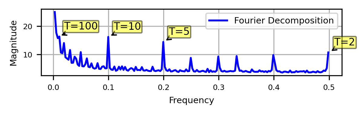
We first Fourier decompose the residual stream after layer 0, and find that the Fourier domain is sparse, with significant high frequency components at $T=[2,5,10]$ and many low frequency components, as shown above. The structure in the Fourier domain implies that numbers are represented with periodic features.

Prior work has also identified these Fourier features, and although initially surprising, are sensible. The units digit of numbers is periodic in base ten ($T=10$), and it is reasonable that qualities like evenness ($T=2$) are useful for tasks as well. However, it is not immediately clear how an LLM could complete a task like greater-than using only Fourier features. We propose additional structure to account for the magnitude of numbers.

Linearity

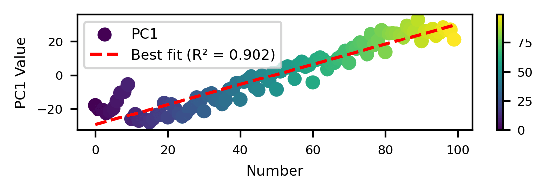
To investigate the additional structure in numbers, we PCA the residual stream and find that the first principal component (PC1) for $a\in [0,360]$ has a sharp discontinuity at $a=100$ which implies that GPT-J uses a distinct representation for three-digit numbers. Instead, we plot PC1 for $a\in [0,99]$ and find that it is well approximated by a line in $a$ (above). The existence of linear structure is unsurprising - numbers are semantically linear, and LLMs often represent concepts linearly. 

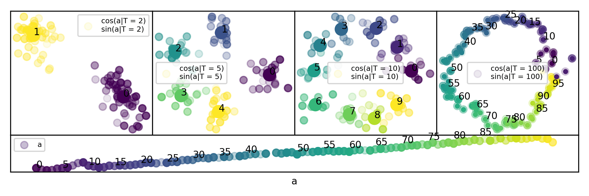
Parameterizing Numbers as a Helix

To account for both the periodic and linear structure in numbers, we propose that numbers can be modeled as a helix. Namely, we posit that $h_a^l$, the residual stream immediately preceding layer $l$ on the token $a$, can be modeled as$h_a^l=helix\left(a\right)=CB(a{)}^T$ with $B\left(a\right)=[a,\cos \left(\frac{2\pi }{T_1}a\right),\sin \left(\frac{2\pi }{T_1}a\right),\dots ,\cos \left(\frac{2\pi }{T_n}a\right),\sin \left(\frac{2\pi }{T_n}a\right)].$

$C$ is a coefficient matrix applied to the basis of functions $B\left(a\right)$, where $B\left(a\right)$ uses $n$ Fourier features with periods $T=[T_1,\dots ,T_n]$.

We identify four major Fourier features: $T=[2,5,10,100]$. We use the periods $T=[2,5,10]$ because they have significant high frequency components. We are cautious of low frequency Fourier components, and use $T=100$ both because it is has significant magnitude, and by imposing the inductive bias that numbers are often represented in base 10 in LLM training data.

Fitting a Helix

We fit our helical form to the residual streams on top of the $a$ token for our $a+b$ dataset. In practice, we first use PCA to project the residual streams at each layer to 100 dimensions. To ensure we do not overfit with Fourier features, we consider all combinations of $k$ Fourier features, with $k\in [1,4]$. If we use $k$ Fourier features, the helical fit uses $2k+1$ basis functions (one linear component, $2k$ periodic components). We then use linear regression to find some coefficient matrix $C_{PCA}$ of shape $100\times 2k+1$ that best satisfies $PCA\left(h_a^l\right)=C_{PCA}B(a{)}^T$. Finally, we use the inverse PCA transformation to project $C_{PCA}$ back into the model's full residual stream dimensionality to find $C$.

We visualize the quality of our fit for layer 0 when using all $k=4$ Fourier features with $T=[2,5,10,100]$ below. To do so, we calculate $C^{†}h$, where $C^{†}$ is the psuedoinverse of $C$. This represents the projection of the residual stream into the helical subspace. The projection looks very pretty and helical:
 

Evaluating the Helical Fit

We want to causally demonstrate that the model actually uses the fitted helix. To do so, we employ activation patching.^[1] Activation patching isolates the contribution of specific model components towards answer tokens by using careful counterfactuals in interventions.^[1]

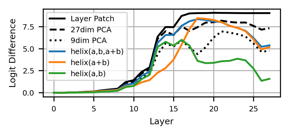
To leverage this technique, we input our fit for $h_a^l$ when patching. This allows us to causally determine if our fit preserves the information the model uses to complete the computation. We compare our helical fit with $k$ Fourier features with four baselines: using the actual $h_a^l$ (layer patch), the first $2k+1$ PCA components of $h_a^l$ (PCA), a circular fit with $k$ Fourier components (circle), and a polynomial fit with basis terms $B\left(a\right)=[a,a^2,...a^{2k+1}]$ (polynomial). For each value of $k$, we choose the combination of Fourier features that maximizes $\frac{1}{L}{\sum }_{l}L{D}_a^l$ as the best set of Fourier features, where $L{D}_a^l$ is the logit difference at layer $l$. 

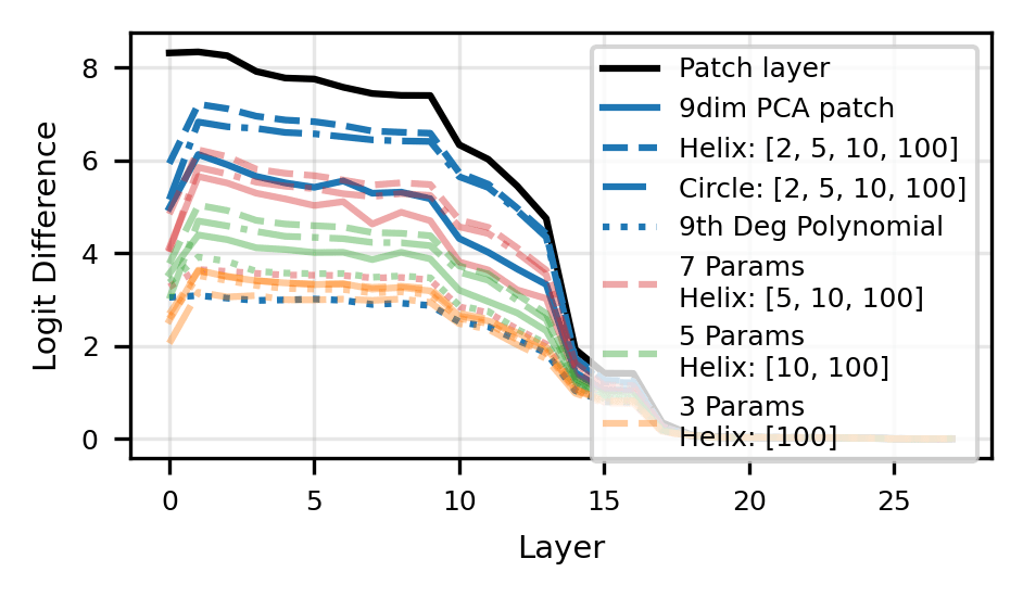
As shown above the helix fit is most performant against baselines, closely followed by the circular fit. This implies that Fourier features are predominantly used to compute addition. Surprisingly, the $k=4$ full helix and circular fits dominate the strong PCA baseline and approach the effect of layer patching, which suggests that we have identified the correct "variables" of computation for addition.

Relation to the Linear Representation Hypothesis^[2] 

We hypothesize that the numerical helix we've identified constitutes a multi-dimensional feature manifold, similar to the one found by Engels, et al. To verfiy this, we adopt the definition of a feature manifold proposed by Olah & Jermyn:

But it may be more natural to understand them as a multidimensional feature if there is continuity. For example, if "midnight on Tuesday" is represented as being between Tuesday and Wednesday, that would seem like some evidence that there really is a continuous representation between them, and cut in favor of thinking of them as a multidimensional feature.

To verify we meet this definition, we first fit all $a$ that do not end with 3 with a $T=100$ helix. Then, we project $a=3,13,\dots ,93$ into that helical space. Below, we find that each point is projected roughly where we expect it to be. For example, 93 is projected between 89 and 95. We take this as evidence that our helices represent a true multidimensional manifold. 

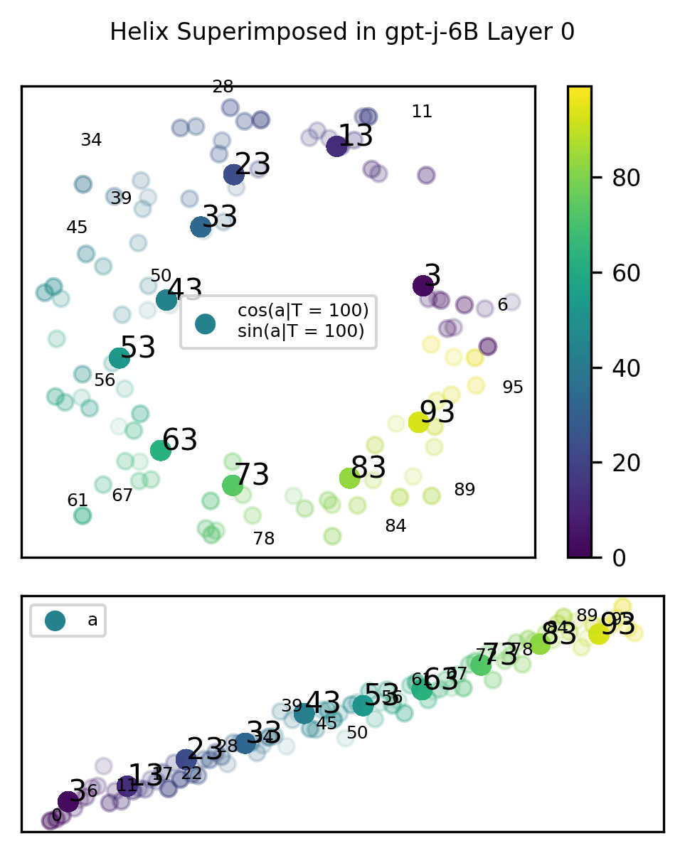
Thus, we find evidence akin to Engels, et al. against the strongest form of the Linear Representation Hypothesis.

Is the helix the full story?

To identify if the helix sufficiently explains the structure of numbers in LLMs, we test on five additional tasks.

1. $a-23$ for $a\in [23,99]$
2. $a//5$ (integer division) for $a\in [0,99]$
3. $a\ast 1.5$ for even $a\in [0,98]$
4. $a\mathrm{mod}2$ for $a\in [0,99]$
5. If $x-a=0$, what is $x=$ for $a\in [0,99]$

For each task, we fit full helices with $T=[2,5,10,100]$ and compare against baselines. 

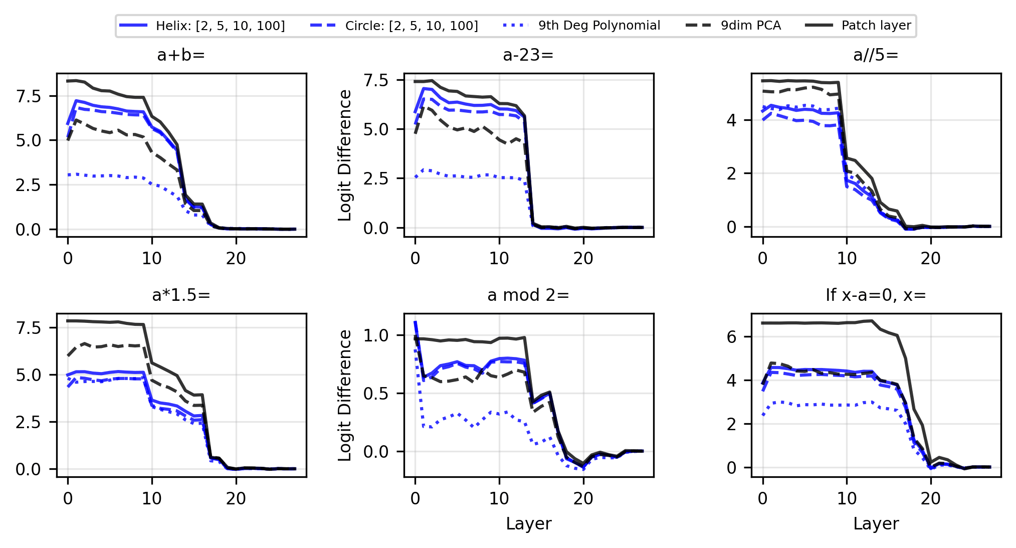
Notably, while the helix is causally relevant for all tasks, we see that it underperforms the PCA baseline on tasks 2, 3, and 5. This implies that there is potentially additional structure in numerical representations that helical fits do not capture. However, we are confident that the helix is used for addition. When ablating the helix dimensions from the residual stream (i.e. ablating $C^{†}$ from $h_a^l$) for addition, performance is affected roughly as much as ablating $h_a^l$ entirely.

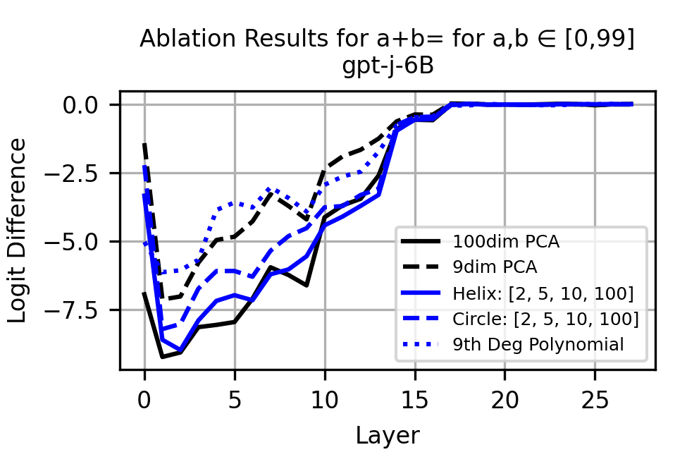
Thus, we conclude that LLMs use a helical representation of numbers to compute addition, although it is possible that additional structure is used for other tasks.

LLMs Use the Clock Algorithm to Compute Addition 

Why would Fourier features be used to compute addition, which is ultimately a linear operation? We hypothesize that they use a form of the Clock Algorithm introduced by Nanda, et al. for one-layer transformers computing modular addition. Specifically, to do $a+b$, we propose that GPT-J

• Embeds $a$ and $b$ as helices on their own tokens.
• A sparse set of attention heads, mostly in layers 9-14, move the $a$ and $b$ helices to the last token.
• MLPs 14-18 manipulate these helices to create the helix $a+b$. A small number of attention heads help with this operation.
• MLPs 19-27 and a few attention heads "read" from the $a+b$ helix and output to model logits.

This algorithm centers on creating $helix(a+b)$ from $helix\left(a\right)$ and $helix\left(b\right)$. Below, we evidence this by the fact that $helix(a+b)$ is a very good fit for the last token residual streams^[3]. In fact, although $helix(a+b)$ uses 9 parameters, it is competitive with a 27 dimensional PCA baseline!

Thus, the crux of the algorithm is creating $helix(a+b)$. Because mostly MLPs are invovled with that operation, in this post we only focus on MLPs. This is supported by the fact that when activation and path patching^[4], we find that MLPs dominate attention heads when measuring causal effect on outputs. For evidence regarding the function of attention heads, please refer to Section 5.2 of the paper.

Understanding MLPs

GPT-J seems to predominantly rely on last token MLPs to compute $a+b$. To identify which MLPs are most important, we first sort MLPs by total effect, and patch in$[1,L=28]$ MLPs to find the smallest $k$ such that we achieve 95% of the effect of patching in all $L$ MLPs. Thus, we use $k=11$ MLPs in our circuit, specifically MLPs 14-27, with the exception of MLPs 15, 24, and 25.

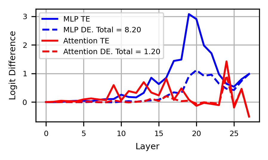
We hypothesize that MLPs serve two functions: 1) reading from the $a,b$ helices to create the $a+b$ helix and 2) reading from the $a+b$ helix to output the answer in model logits. We make this distinction using two metrics: $helix(a+b)$/TE, or the total effect of the MLP recoverable from modeling its output with $helix(a+b)$, and DE/TE ratio. 

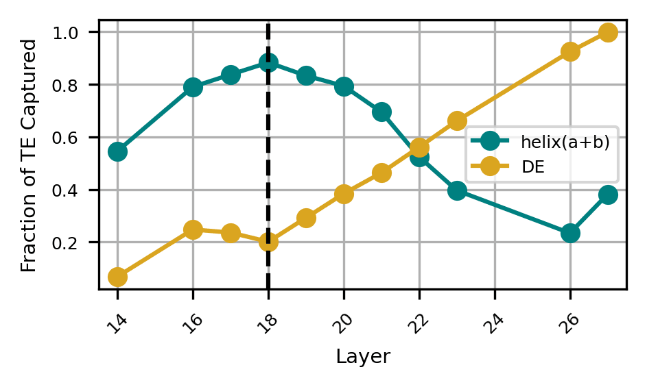
Above, we see that the outputs of MLPs 14-18 are progressively better modeled using $helix(a+b)$. Most of their effect is indirect and thus their output is predominantly used by downstream components. At layer 19, $helix(a+b)$ becomes a worse fit and more MLP output affects answer logits directly. We interpret this as MLPs 14-18 "building'" the $a+b$ helix, which MLPs 19-27 translate to the answer token $a+b$.

However, our MLP analysis has focused solely on MLP outputs. To demonstrate the Clock algorithm conclusively, we must look at MLP inputs: neurons.

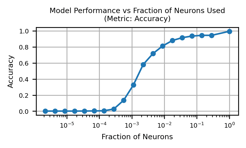
Zooming in on Neurons

Activation patching the $27\ast 16384$ neurons in GPT-J is prohibitively expensive, so we instead use the technique of attribution patching to approximate the total effect of each neuron using its gradient^[5]. We find that using just 1% of the neurons in GPT-J and mean ablating the rest allows for the successful completion of 80% of prompts. Thus, we focus our analysis on this sparse set of $k=4587$ neurons.

Modeling Neuron Preactivations

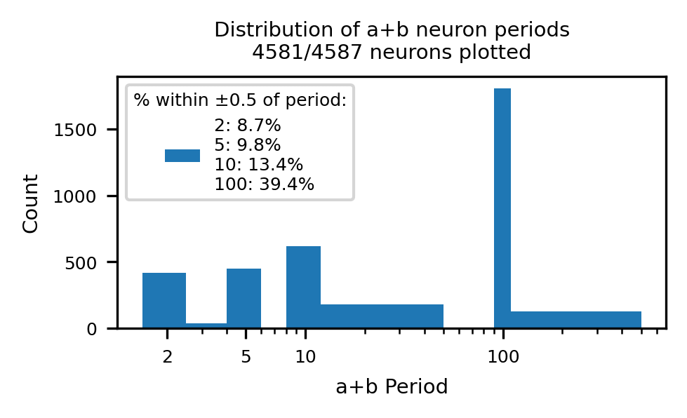
For a prompt $a+b$, we denote the preactivation^[6] of the $n$th neuron in layer $l$ as $N_n^l(a,b).$ When we plot a heatmap of $N_n^l(a,b)$ for top neurons below, we see that their preactivations are periodic in $a,b$, and $a+b$. 

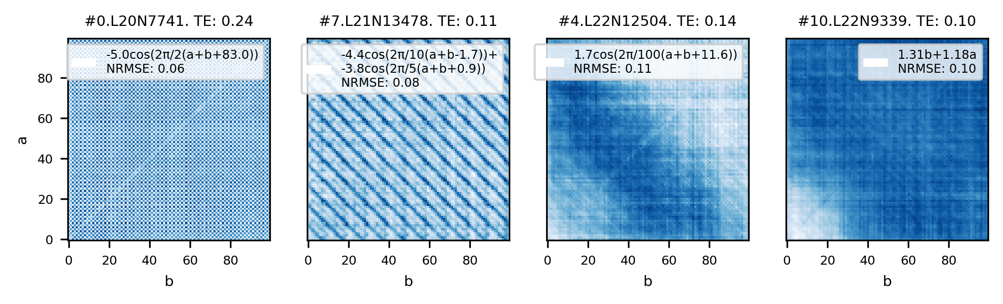
When we Fourier decompose the preactivations as a function of $a+b$, we find that the most common periods are $T=[2,5,10,100]$, matching those used in our helix parameterization. This is sensible, as the $n$th neuron in a layer applies $W_{up}^n$ of shape $(4096,)$ to the residual stream, which we have effectively modeled as a $helix(a,b,a+b)$. 

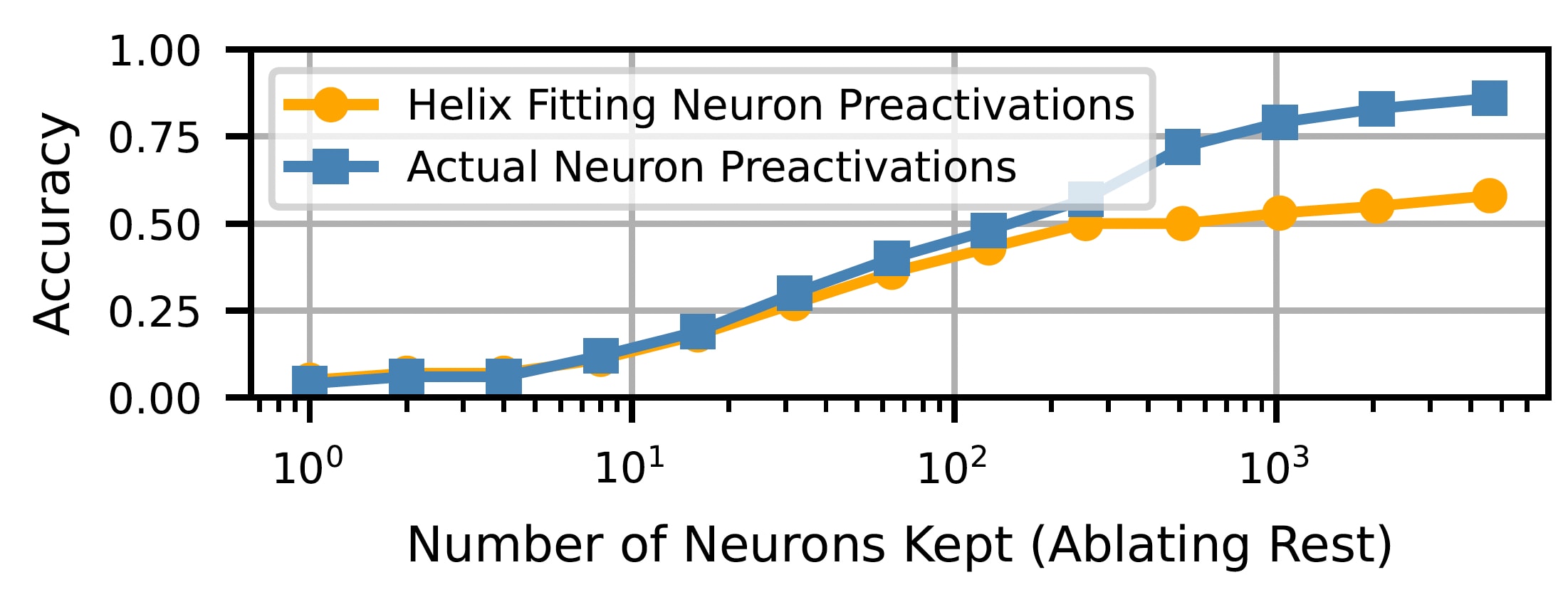
Subsequently, we model the preactivation of each top neuron as

$N_n^l(a,b)={\sum }_{t=a,b,a+b}{c}_{t}t+{\sum }_{T=[2,5,10,100]}{c}_{Tt}\cos \left(\frac{2\pi }{T}\right(t-d_{Tt}\left)\right)$

See examples of the fits used in the legend of the previous preactivation figure. We fit the $k=4587$ identified neurons, and plug these fits back into the model. We mean ablate all other neurons. We find that using these helix inspired fits recover most of the performance of using the actual preactivations!

Understanding MLP Inputs

We use our understanding of neuron preactivations to draw conclusions about MLP inputs. To do so, we first path patch each of the top $k$ neurons to find their direct effect and calculate their DE/TE ratio. For each neuron, we calculate the fraction of their fit that $helix(a+b)$ explains, which we approximate by dividing the magnitude of $c_{T,a+b}$ terms by the total magnitude of $c_{Tt}$ terms in the preactivation fit equation. For each circuit MLP, we calculate the mean of both of these quantities across top neurons.

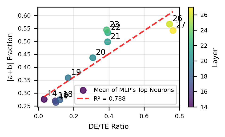
Once again, we see a split at layer 19, where earlier neurons' preactivation fits rely on $a,b$terms, while later neurons use $a+b$ terms and write to logits. Since the neuron preactivations represent what each MLP is "reading'" from, we combine this with our understanding of MLP outputs to summarize the role of MLPs in addition.

• MLPs 14-18 primarily read from the $a,b$ helices to create the $a+b$ helix for downstream processing.
• MLPs 19-27 primarily read from the $a+b$ helix to write the answer to model logits.

Thus, we conclude our case that LLMs use the Clock algorithm to do addition.

Interpreting Model Errors

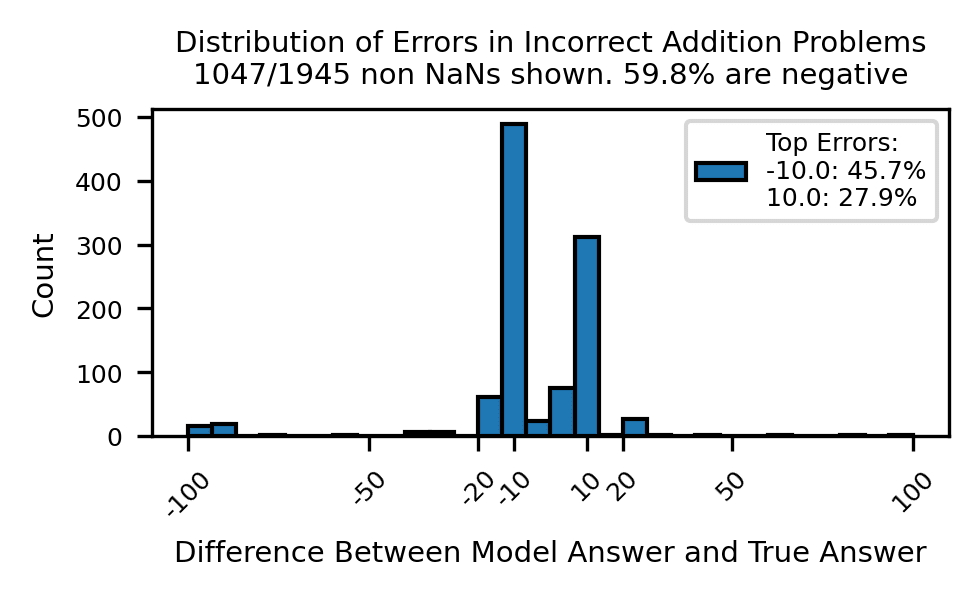
Given that GPT-J implements an algorithm to compute addition rather than relying on memorization, why does it still make mistakes? For problems where GPT-J answers incorrectly with a number, we see that it is most often off by -10 (45.7%) and 10 (27.9%), cumulatively making up over 70% of incorrect numeric answers. We hypothesize that reading from the $a+b$ helix to answer logits is flawed.^[7]

Since MLPs most contribute to direct effect, we begin investigating at the neuron level. We sort neurons by their direct effect, and take the $k=693$ highest DE neurons required to achieve 80% of the total direct effect. Then, we use the technique of LogitLens to understand how each neuron's contribution boosts and suppresses certain answers^[8]. For the tokens $[0,198]$(the answer space to $a+b$), we see that each top DE neuron typically boosts and suppresses tokens periodically.

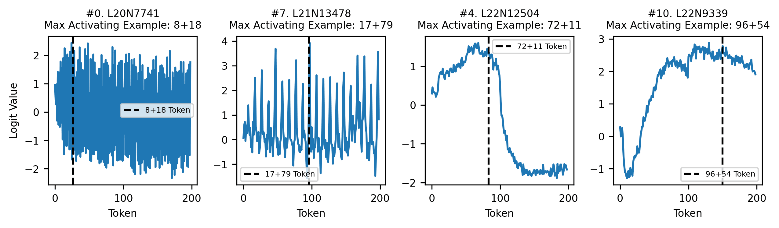
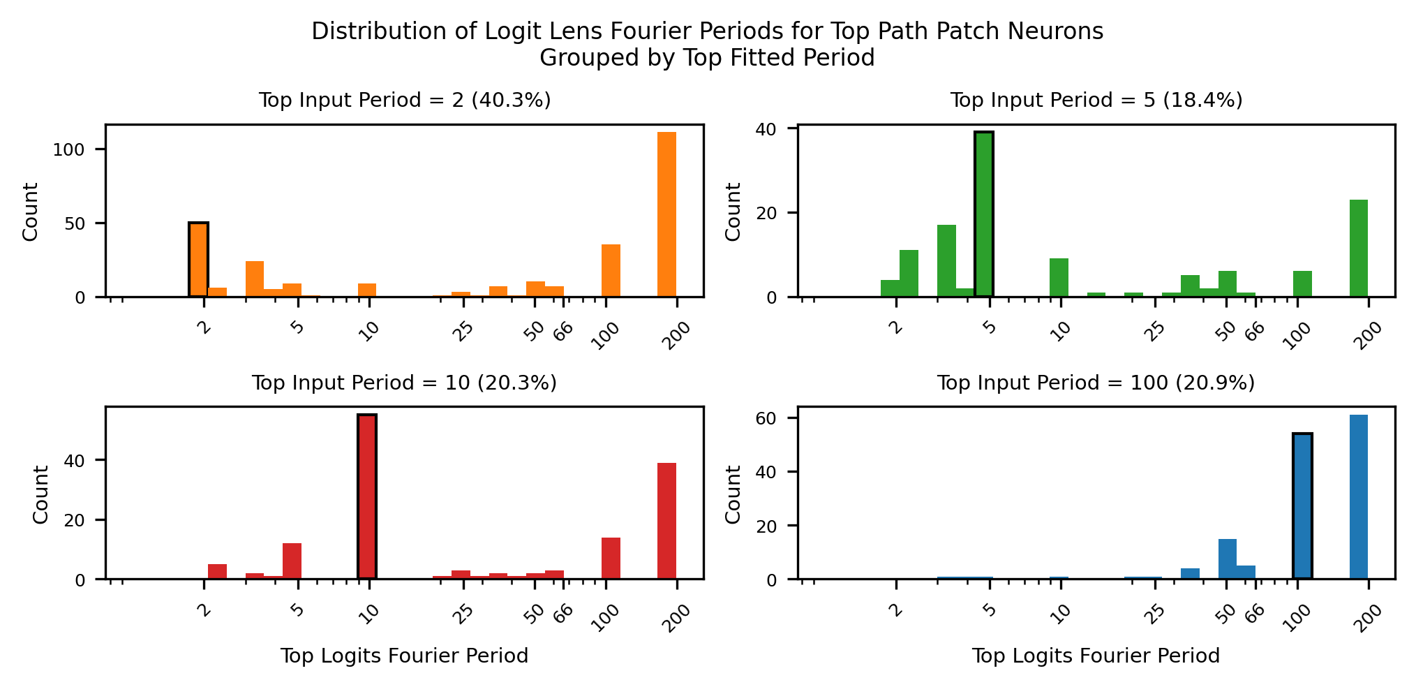
Moreover, when we Fourier decompose the LogitLens of the max activating $a+b$ example for each neuron, we find that a neuron whose preactivation fit's largest term is $c_{T_i,a+b}$ in its preactivation fit often has LogitLens with dominant period of $T_i$ as well. We interpret this as neurons boosting and suppressing tokens with a similar periodicity that they read from the residual stream helix with.

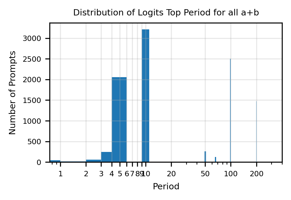
Despite being periodic, the neuron LogitLens are complex and not well modeled by simple trigonometric functions. Instead, we turn to more broadly looking at the model's final logits for each problem $a+b$ over the possible answer tokens $[0,198]$. We note a similar distinct periodicity.

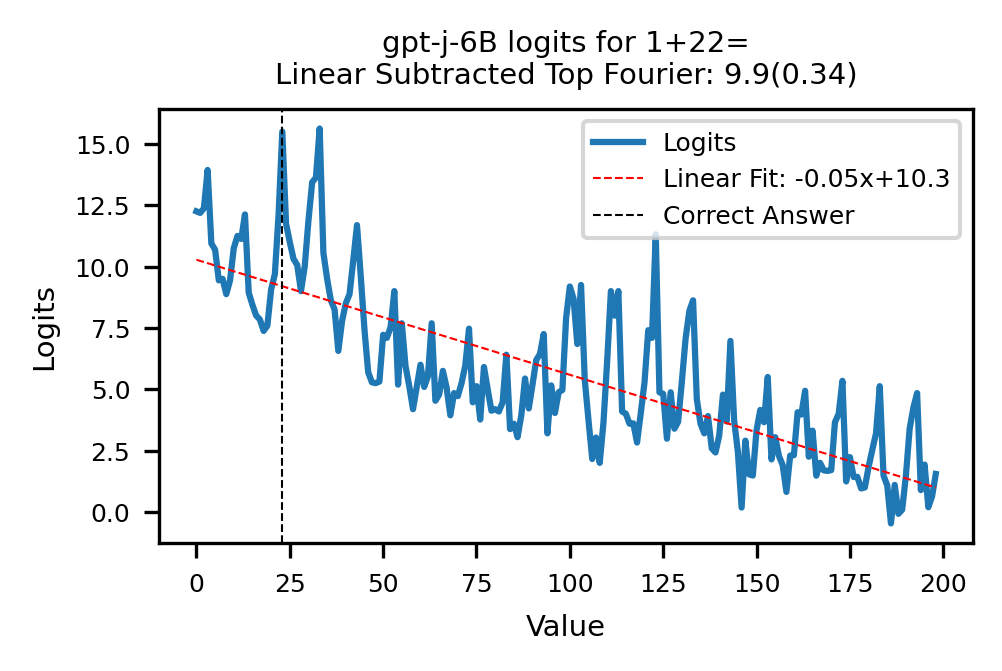
When we Fourier decompose the logits for all problems $a+b$, we find that the most common top period is 10. Thus, it is sensible that the most common error is $\pm 10$, since $a+b-10$, $a+b+10$ are also strongly promoted by the model. 

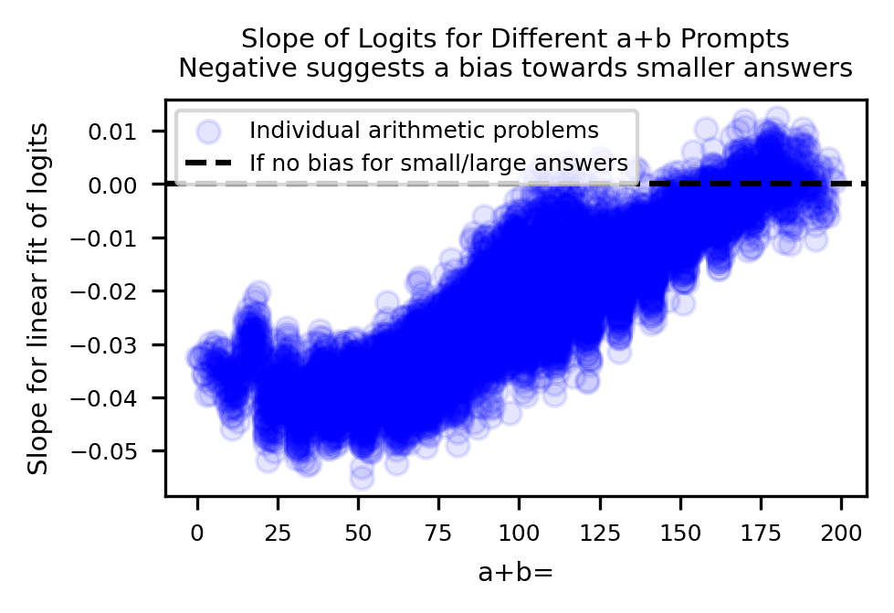
To explain why -10 is a more common error than 10, we fit a line of best fit through the model logits for all $a+b$, and note that the best fit line almost always has negative slope indicating a preference for smaller answers. This bias towards smaller answers explains why GPT-J usually makes mistakes with larger $a$ and $b$ values.

Limitations

There are several aspects of LLM addition we still do not understand. Most notably, while we provide compelling evidence that key components create  $helix(a+b)$ from $helix(a,b)$, we do not know the exact mechanism they use to do so. We hypothesize that LLMs use trigonometric identities like $\cos (a+b)=\cos \left(a\right)\cos \left(b\right)-\sin \left(a\right)\sin \left(b\right)$ to create $helix(a+b)$. However, like the originator of the Clock algorithm, we are unable to isolate this computation in the model. This is unsurprising, as there is a large solution space for how models choose to implement low-level details of algorithms. 

Additonally, while our results for GPT-J and Pythia-6.9B are strong, our results for Llama3.1-8B are weaker. For instance, $helix(a+b)$ is a considerably worse fit on last token hidden states.

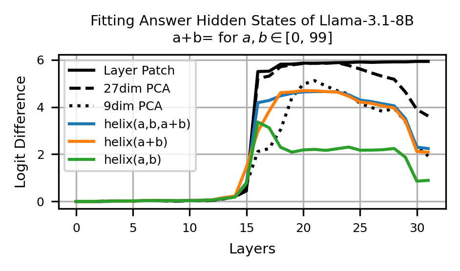
We consider it likely that LLMs use multiple algorithms coupled together, and hypothesize that Llama3.1-8B's use of gated MLPs makes it prefer other addition algorithms that the simple of MLPs of GPT-J and Pytha-6.9B don't use. Additionally, this study has focused on models with single-token representations of two digit numbers. A model like Gemma-2-9B uses single-digit tokenization and likely requires additional algorithms to collate digits together into a single numerical representation.

Conclusion

We find that three mid-sized LLMs represent numbers as helices and manipulate them using the interpretable Clock algorithm to compute addition. It is remarkable that LLMs trained on simple next token addition learn a complex algorithm for a task like addition instead of just memorizing the training data. We find it especially interesting that they use roughly the same algorithm used by a one layer transformer, providing hope that our understanding of small models can scale to larger ones. We hope that this work inspires additional investigations into LLM mathematical capabilities, especially as addition is implicit to many reasoning problems. 

1. ^{^}

   Specifically, to evaluate the contribution of some residual stream $h_a^l$ on the $a$ token, we first store $h_{a,\text{clean}}^l$ when the model is run on a "clean'" prompt $a+b$. We then run the model on the corrupted prompt $a^{\prime }+b$ and store the model logits for the clean answer of $a+b$. Finally, we patch in the clean $h_{a,\text{clean}}^l$ on the corrupted prompt $a^{\prime }+b$ and calculate $L{D}_a^l=logi{t}_{patched}(a+b)-logi{t}_{corrupted}(a+b)$, where $L{D}_a^l$ is the logit difference for $h_a^l$. By averaging over 100 pairs of clean and corrupted prompts, we can evaluate $h_a^l$'s ability to restore model behavior to the clean answer $a+b$.

2. ^{^}

   The Linear Representation Hypothesis posits that LLMs store features as linear directions in activation space.

3. ^{^}

   Note that $helix(x,y)$ is shorthand to denote $helix\left(x\right)+helix\left(y\right)$.

4. ^{^}

   Path patching isolates how much components directly contribute to logits. For example, MLP18's total effect (TE, activation patching) includes both its indirect effect (IE), or how MLP18's output is used by downstream components like MLP19, and its direct effect (DE, path patching), or how much MLP18 directly boosts the answer logit.

5. ^{^}

   See Nanda.

6. ^{^}

   Recall that GPT-J uses a simple MLP: $MLP\left(x\right)=\sigma \left(x{W}_{up}\right)W_{down}$. $x$ is a vector of size $(4096,)$ representing the residual stream, and $W_{up}$ is a $(4096,16384)$ projection matrix. The input to the MLP is thus the 16384 dimensional $x{W}_{up}$. We denote the $n$th dimension of the MLP input as the $n$th neuron preactivation.

7. ^{^}

   In Appendix F, we consider and falsify the hypothesis that the model is failing to "carry" the 10s digit when constructing $helix(a+b)$.

8. ^{^}

   See nostalgebraist [LW · GW] for details.

0 comments

Comments sorted by top scores.