Transformers Explained (Again)

rohans

Transformers Explained (Again)

post by RohanS · 2024-10-22T04:06:33.646Z · LW · GW · 0 comments

  Introduction
  Inputs and Outputs
  Exploring Model Internals
    Preface: Loss function and grouping components
    Tracing the path of an input through a transformer
  Summary
  References
None
No comments

I actually wrote this in Spring 2023. I didn't post then because I had trouble converting this Google doc to any other format; the Lesswrong gdoc import feature made that easy. :)

Introduction

This is yet another post about the Transformer neural network architecture, written in large part for my own benefit. There are many other resources for understanding transformers, and you may be better off using one of them. However, I will emphasize some of the things that I did not fully understand after reading a few posts and watching a few videos about transformers, so this could potentially still be useful to people. I filled in a lot of the remaining gaps by watching this video by Neel Nanda and writing all the code to follow along with it myself (though that took a while). The video focuses on a GPT-2 style (decoder-only) transformer, and that is also what this post will focus on.

Inputs and Outputs

This section doesn’t say anything about the internals of the transformer architecture, but it contains a lot of the information relevant to transformer models that took me the longest to figure out.

Input: Natural language string. E.g. “The development of Artificial General Intelligence (AGI) may well be the most important event in human”
- Let me address some possible confusions with this input:
  - It is not a complete sentence. This is because the transformer’s job, as we will see below, is to predict the next token, and I wanted to give an example where there is an expected output (“ history”, with a leading space).
  - It only includes a single string, and the model can actually run on a batch of strings at a time (a single string is a special case where batch_size=1).
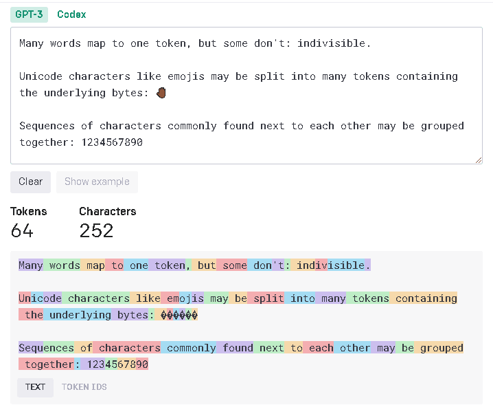
  - Natural language strings don’t actually get passed into transformers. Instead, a natural language string gets turned into a list of tokens, where tokens correspond to words or short strings of letters within words.
    - Example from here:

The set of all possible tokens is called the model’s vocabulary. The way the vocabulary is constructed is interesting and worth understanding - let’s discuss that now.
- The method for constructing the vocabulary is called Byte-Pair Encoding (BPE).
- First, we initialize the vocabulary with all 256 ASCII characters in it. Note that this means it is possible to decompose or construct any text string, including nonsense strings of symbols that are never seen during training, with tokens in the vocabulary, since each character can be a separate token.
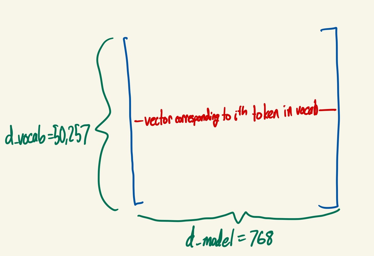
- Then, BPE looks through the training data for the most common character sequences that aren’t already in the vocabulary. The most common two character string is “ t” (a space followed by a t), so that is added to the vocabulary. BPE continues adding common strings to the vocabulary until some preset vocab size limit is reached. We call this vocab size d_vocab: d_vocab = 50,257 for GPT-2, and I think GPT-3 as well.
- It’s possible this isn’t a perfect description of BPE, but conceptually the idea that the vocab contains the most common character strings (including all single-character strings) is correct.
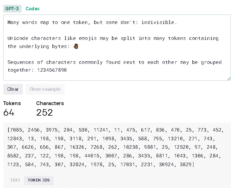
  - The list of tokens can then easily be converted into a list of integers, where each integer corresponds to the index of the token in the vocabulary.
    - Example (compare to the image above):

Actual input: Tokens. More specifically, a list of integers corresponding to the indices in the vocab of the tokens that compose the natural language string above.
- Shape: [batch, position] (The tensor has “batch” elements along the first dimension and “position” elements along the second dimension, where “batch” and “position” are numbers. For the purposes of this post, and I think much of deep learning, “tensor” just means “array with any number of dimensions.”)
  - “batch” is short for batch_size.
  - “position” refers to the fact that the integer at index i along that dimension corresponds to the token at position i in the input string. In my opinion calling this position is a little confusing, so let’s interpret it carefully and consider alternative names for it (though we’ll continue to use “position” below, since that is what Neel Nanda called it in the video and he probably knows better than I do).
    - One possible alternative for “position” could be “tokens” (resulting in [batch, tokens]), since the size of the input along this dimension is the number of tokens in the input string. This gets confusing when there is more than one input string in the batch, i.e. batch_size > 1. What is the size of the input along the second dimension in that case? The next alternative makes this clear.
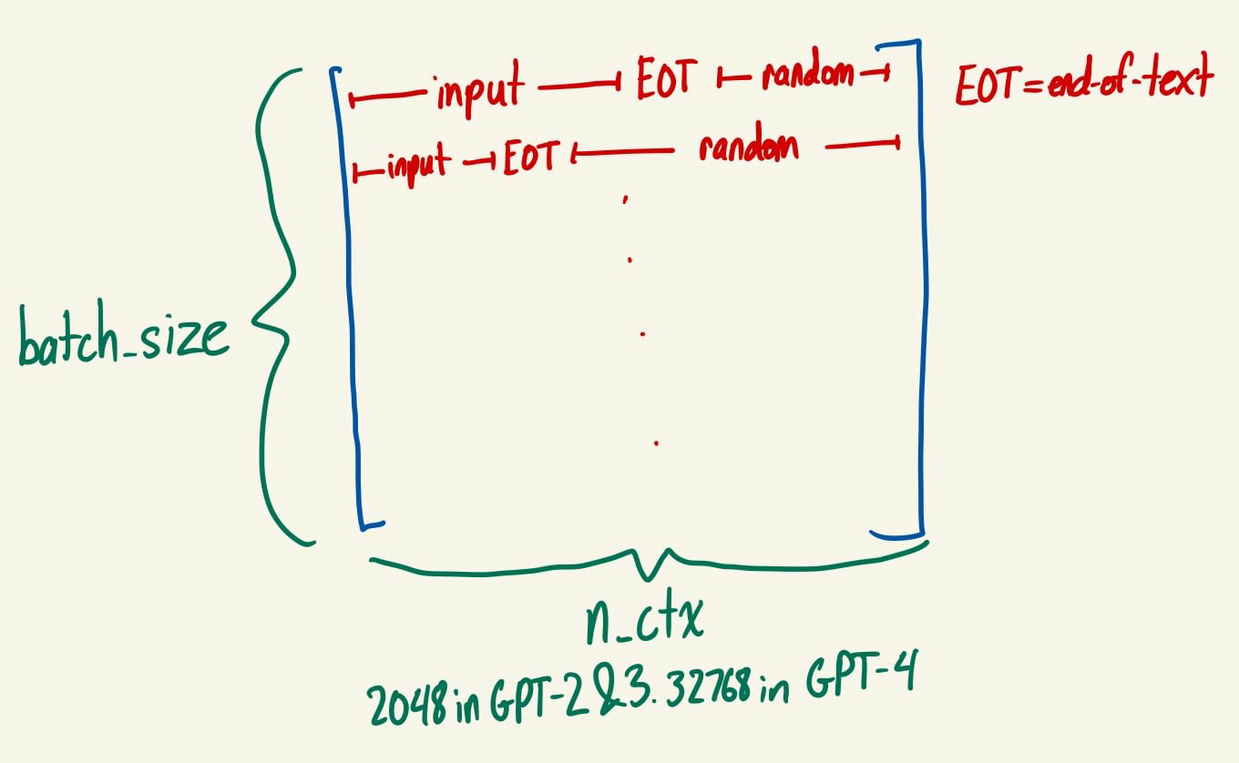
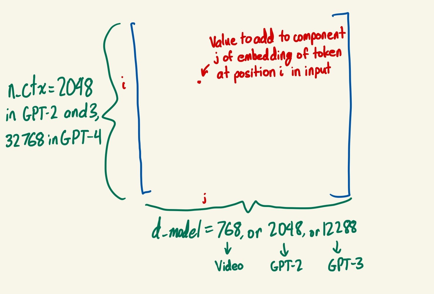
    - “n_ctx” is another possible alternative for “position” when batch_size > 1. n_ctx is the maximum number of tokens that the model can handle as input: In GPT-2 and GPT-3, n_ctx = 2048. GPT-4 has n_ctx = 32,768. This is called the size of the context window. As noted above, it is unclear how many elements there should be along the second dimension of this tensor when there are multiple inputs of different lengths within a batch. Instead of having a different number of elements for each input, we can use n_ctx for all inputs, since no input string has more than n_ctx tokens. I believe the end of the actual input is demarcated by a special end-of-text token which tells the model to ignore all the random tokens that come afterward, but I’m not 100% sure about this.

Output: The transformer runs on the input and generates a logits vector for each position in each input of the batch. This logits vector can be converted into a vector of probabilities with a softmax. (It’s definitely important to understand softmax well in order to understand transformers, so I suggest reading that link now if you aren’t familiar. It’s pretty short.) The ith probability in the vector of probabilities for position j is the probability the model assigns to the ith token in its vocabulary being the next token after the input token at position j, i.e. the token at position j+1 in the input. We are often particularly interested in predicting what comes after the whole input, so we are often most interested in the probabilities that the model assigns to the token after the final token of the input. If the model is doing a good job (and the input is a reasonable sentence), then hopefully it assigns high probability to the actual next token in the input for all other positions. (It isn’t allowed to “peek” at the token at position j+1 when predicting it, so this is not trivial. I will elaborate on this later - the relevant term to look out for is “causal mask.”)
- Shape: [batch, position, d_vocab]
  - Reminder: d_vocab is the number of tokens in the model’s vocabulary.
- Consider the example input string from above, “The development of Artificial General Intelligence (AGI) may well be the most important event in human”. If this is converted into a list of tokens and passed into a good transformer model, the output at the last position will be a logits vector whose largest element is at index i, where i is the index of “ history” (with a leading space) in the model’s vocabulary (assuming “ history” is a token in the vocab).
  - (The index of the largest logit is the same as the index of the largest probability after taking a softmax.)
Generating text: The (main) output of the transformer model is a logits vector that yields the probability associated with any given token appearing next. How can this be converted into actual text? For instance, how does something like ChatGPT generate extended text responses?
- There are many methods available for this. The most obvious one is greedy text generation: Select the most likely next token, append it to the input string, run the model on this new string, append the token that run finds most likely, and continue repeating this procedure.
- Beam search is another common method. You can read more about that and several other methods in this article. Greedy is the simplest, but not the best: it helps to be able to consider which words to say together, instead of just picking the best next word at any given time.

Exploring Model Internals

Preface: Loss function and grouping components

Note that nothing described in the previous section involves learning parameters. That’s because we’ve only discussed the inputs and the outputs of the model, not its internal structure. We’ve already had to do quite a bit of manipulation on both ends, but the model details are yet to come.

We start with a randomly initialized model with a structure we have imposed, and then we tune parameters within that structure to perform a task well. This post is trying to elucidate “the structure we have imposed,” because that is what the Transformer architecture is. I find it useful to take careful note of what things receive random initializations, because those things do not intrinsically serve a certain purpose - instead, they learn to serve a certain purpose because of the way they are used.

Let’s focus on the loss function used to train GPT-2 in order to understand the task it is trained to perform. It is an autoregressive language model, which means that given a sequence of tokens, it predicts the next token. This is sometimes called “causal language modeling.” The reason for this is something like “only tokens before the token-to-be-predicted can have a causal influence on the model’s prediction.” An alternative is “masked language modeling,” which involves selecting a token to insert into a missing space in a sequence of tokens. BERT is a popular model trained on a masked language modeling objective.

The way (or at least, one way) to train an autoregressive language model is as follows. Start with all parameters of the model randomly initialized. Run the model on an input string where you know what the next token should be. Apply a softmax to the logits vector it produces, so we have the probability the model assigns to each possible next token. Extract the probability assigned to the correct next token. Take the logarithm of this probability, then negate it. This is the loss associated with this model output. Use backpropagation and stochastic gradient descent (SGD) to train the model using this loss.

More concisely: Loss = -log(softmax(logits)[correct_token_index])

softmax(logits) is the vector of probabilities
softmax(logits)[correct_token_index] is the probability assigned to the correct token.
This is the loss on a single input. In practice, we want to do this a batch at a time, so that involves taking the average single-input loss across all inputs in the batch.
This is called cross-entropy loss. Cross-entropy loss more generally is of the form Loss = $- | Y | \sum i = 1 y_{i} log {^y}_{i}$ , where Y is the set of output features, $y_{i}$ is the ground truth label for output feature i, and ${^y}_{i}$ is the model’s predicted value for output feature i. Here, the ground truth label $y_{i}$ = 0 for every i other than the index of the correct next token in the vocab, and $y_{i}$ = 1 for that index, so the loss is just the negation of the log of the probability assigned by the model to the correct token.

What’s going on here? Minimizing the loss is equivalent to maximizing the probability that the model assigns to the correct next token, since the loss is equal to the negative log probability assigned and log is monotonically increasing (i.e. if you increase x, log(x) also increases). I believe the log is included in the loss because that makes computing derivatives of the loss (with respect to the model parameters) tractable, which is necessary for training the model using SGD and backpropagation.

Now that we understand the loss function, we know that the trainable parameters of a GPT-2 style transformer model are randomly initialized and then slowly adjusted to perform the task of next-token prediction more effectively.

Before finally seeing what happens to an input as it passes through a transformer, there is one meta-level point about understanding this that I want to make. Part of the difficulty of understanding transformer models is in figuring out how “zoomed in” you are supposed to be - that is, how many parts of the model do you have to pay attention to at the same time in order to understand what’s going on? Which ones have functions that are detached enough from each other that you can look at them separately? Here is a quick walkthrough of the components of a transformer model with my answers to these questions - everything will be explained in more depth in the next section.

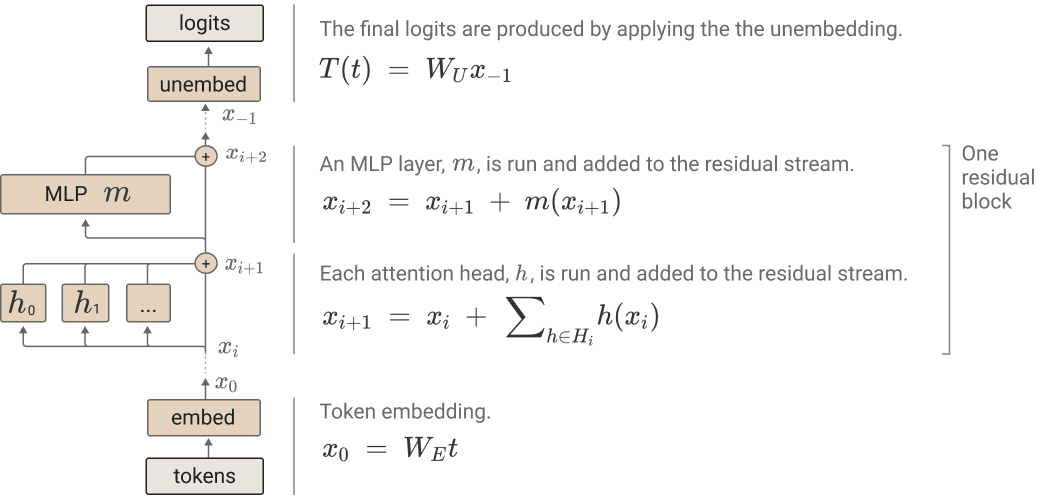
(Read this image from bottom to top, and use the text below to clarify things.)

First, tokens are passed through an embedding layer, which can be considered by itself.
Next, there is a positional embedding layer (not in the image), which can also be considered by itself.
After that there are many residual blocks (96 in the case of GPT-3), also called transformer blocks. You should, by the end of this post, be able to view a transformer block as a single entity, while also understanding its component parts. Once you understand transformer blocks, it should be fairly intuitive that stacking a lot of them back to back can create a powerful model.
- The first breakdown of a transformer block is into a layer normalization layer (LayerNorm), followed by an attention layer, then another LayerNorm, and then an MLP (multilayer perceptron, or vanilla neural network).
  - LayerNorm normalizes the input it receives, and can be understood in isolation.
  - Each attention layer is composed of many attention heads (also 96 in GPT-3). Understanding attention heads by themselves is a bit of a challenge. Four separate linear maps are learned within each attention head.
    - Three of them are applied to the input: A query linear map produces queries, a key linear map produces keys, and a value linear map produces values. The context for these linear maps is provided in the next two bullets.
    - Queries and keys are combined in a specific way (which will be described in detail below) to produce attention probabilities. This step can partially be viewed in isolation, and should also be understood in the context of how the attention probabilities are used.
    - These attention probabilities are used to take a weighted average of the values. This step can be viewed in isolation.
    - The fourth linear map is an output linear map which maps the weighted average of the values to the output of the attention head. This step can be understood in isolation.
    - The output of an attention layer is the sum of the outputs of all its attention heads. This output is added to the input that the attention layer received and passed on to the next part of the model. The fact that the previous input is always kept and added to means that information from earlier in the model is never completely lost. We say that the model has a residual stream, and attention layers (and MLP’s, as we will see) pass information onward by adding it to the residual stream.
  - Another LayerNorm is applied to the residual after the output of the attention layer is added.
  - The residual is then passed through an MLP. Hopefully you already understand MLP’s - if not, this video is a pretty good way to learn about them. The output of the MLP is added to the residual stream.
- Transformer blocks are executed in sequence, taking the output of the preceding one as input.
After all transformer blocks have been completed, a final LayerNorm is applied to produce a final normalized residual vector.
Then, an unembedding layer converts the final residual into the final model output, which are logits as discussed above.

It’s fine if not everything here makes sense yet. Hopefully reading the next section will make things much clearer, and you can refer back to this overview to check if it is starting to make sense. This overview is the collection of high-level concepts that I want you to store as a compressed understanding of transformers at the end of this post, but you need to see the low-level details in order for the high-level summary to really make sense.

Tracing the path of an input through a transformer

Input: Tokens. More specifically, a list of integers corresponding to the indices in the vocab of the tokens that compose the natural language string above.
- Shape: [batch, position]
- Recall the discussion in the Inputs and Outputs section above.
Embedding: The tokens are embedded into the vector space $R^{d_{m o d e l}}$ . In GPT-2, d_model = 2048. In GPT-3, d_model = 12288. It is just a lookup table: a separate vector is learned for every token.
- embed = Embed(tokens)
  - Shape: [batch, position, d_model]
  - embed can be considered the first residual vector, and this can be considered the beginning of the residual stream.
  - If you iterate over the batch dimension, you are looking at different inputs. If you iterate over the position dimension for a given input, you are looking at different positions in that input. If you iterate over the d_model dimension for a given input and token, you are looking at the components of the embedding vector for that token.
    - There is nothing particularly special about any particular value of d_model: $R^{d_{m o d e l}}$ is just a vector space in which the model can perform computations. The larger d_model is, the more complex relationships can be stored.
- A d_vocab x d_model matrix is randomly initialized. Forward passes of the model use this matrix by replacing each token index i in the input (corresponding to the ith token in the vocabulary) with the ith row vector in the matrix - that’s what embedding means. Therefore, the model learns a matrix such that the relationships between the row vectors reflect the relationships between the corresponding words.
- - d_model = 768 in the model I wrote while following the Neel Nanda video, which is a smaller version of GPT-2 (maybe exactly the model called GPT-2 Small). Again, in GPT-2, d_model = 2048, and in GPT-3, d_model = 12288.
  - Note that this isn’t a matrix that does any multiplications - it is just a lookup table. If token i in the vocab is in the input, you look up the ith row of this matrix and use it.
- A classic example of a semantic relationship in embeddings:
  - Let E(w) be the embedding (a vector) for the word w. E(king) - E(man) + E(woman) might give you (something very close to) E(queen).
    - I’m fairly sure this is a classic example because some researchers actually found this to be the case in some model, though I think that was with a different embedding scheme, before transformers existed or became popular.
  - More discussion of language embedded into vector spaces here.
Positional Embedding: Add a learned value at each token position and residual component to give the model an indication of where in the sentence each token appeared.
- pos_embed = PosEmbed(embed)
  - Shape: [batch, position, d_model]
- An n_ctx x d_model matrix is randomly initialized. During forward passes of the model, the ij entry of this matrix is added to location [input,i,j] of the embed tensor for all inputs (so the contribution of the positional embedding is the same for all inputs), for all i and j.
- Note that this also isn’t a matrix that does any multiplications - it just adds something at each position and d_model component.
- It’s not clear to me how important positional embeddings are for transformers to function effectively: I believe there has been some work exploring how they do without positional embeddings, but I don’t know the results. The basic argument for the usefulness of positional embeddings is that it provides the model with some information about where in the input each token appeared, which seems useful for predicting next tokens.
residual = embed + pos_embed
- Shape: [batch, position, d_model]
- pos_embed is a function of embed, and then we add it to embed again. This is standard for the residual stream: we take some residual vector (e.g. embed), transform it in some way (e.g. pos_embed = PosEmbed(embed)), and add the result back to the original residual vector (e.g. residual = embed + pos_embed). This pattern will be repeated many times below.
Transformer Block #1: Takes residual as input.
- LayerNorm: Normalize residual to have mean 0 and variance 1, then multiply it by some learned weights and add a learned bias.
  - normalized_resid_pre = LN(residual)
    - Shape is still [batch, position, d_model]
  - Fix a specific position in a specific input in residual. The vector (of dimension d_model) at that position in that input gets normalized as follows:
    - Take the mean value of the d_model components of the vector, and subtract it from every component. Now the mean value of all the components is 0.
    - Take the standard deviation of the components of the (mean 0) vector and divide every component by that standard deviation. Now the standard deviation is 1 (as is the variance). Call this the new normalized vector.
    - A weights vector of dimension d_model is randomly initialized. (These weights are learned during training.)
      - Multiply every component of the normalized vector by the corresponding weight in the weights vector; that is, multiply normalized[i] by weights[i], for all i between 0 and d_model-1. Call this the weighted normalized vector.
    - A biases vector of dimension d_model is randomly initialized. (These biases are learned during training.)
      - Add every bias in the biases vector to the corresponding component in the weighted normalized vector; that is, add biases[i] to weighted_normalized[i], for all i between 0 and d_model-1.
  - The above operations are performed for every input and position.
- Attention Layer: Takes normalized_resid_pre as input.
  - Attention Heads: GPT-3 has 96 attention heads per attention layer, GPT-2 small has 12. I will now describe what happens in a single attention head; the only difference between them is that they have separate learnable parameters. The input to each is still normalized_resid_pre.
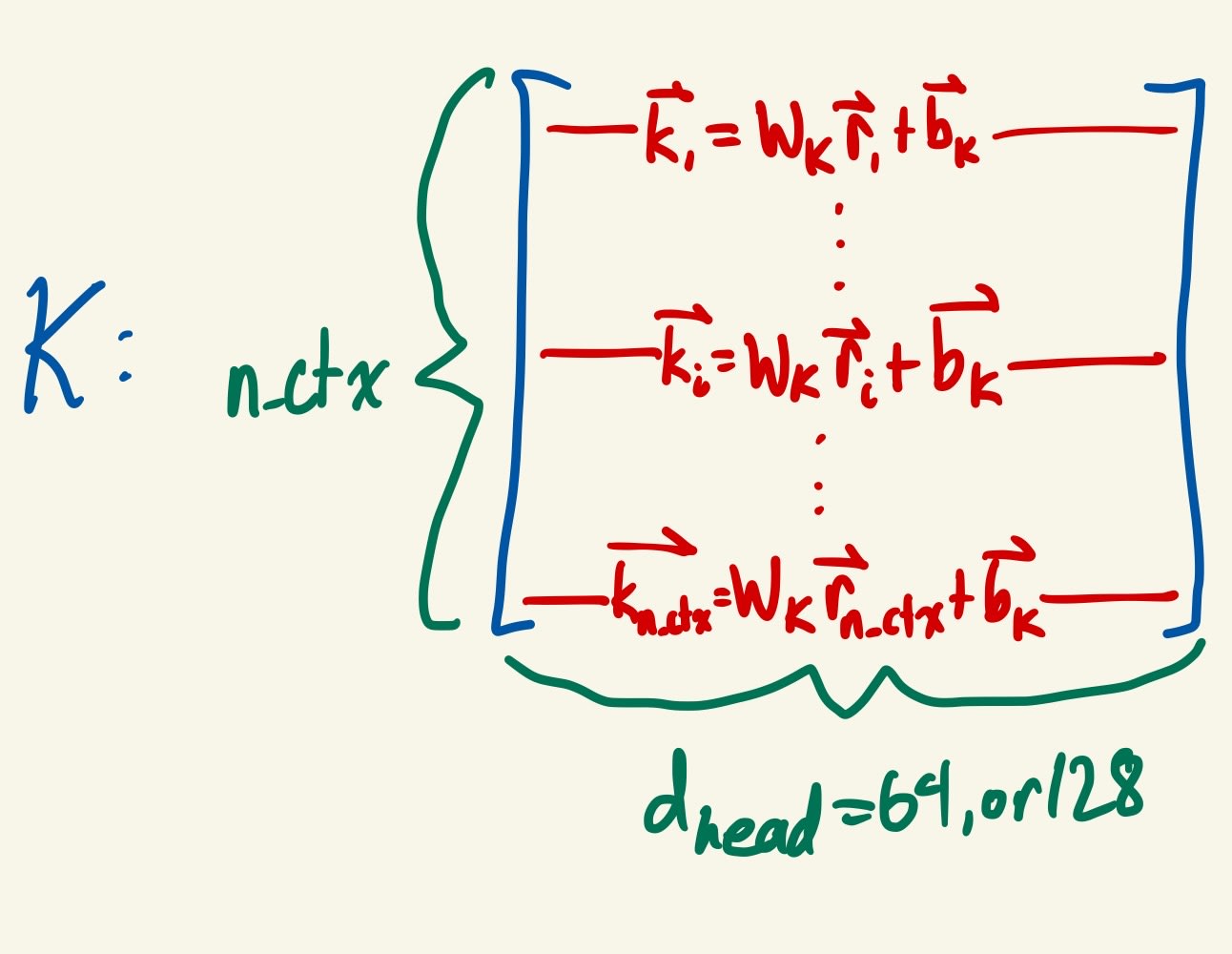
    - 3 matrices of shape d_head x d_model are randomly initialized. (Like d_model, there is nothing special about any particular value for d_head: $R^{d_{h e a d}}$ is just a vector space in which the model can perform computations. d_head = 64 in GPT-2 Small and 128 in GPT-3.) Call these 3 matrices WQ (query matrix), WK (key matrix), and WV (value matrix). 3 vectors of dimension d_head are randomly initialized: call them bQ, bK, and bV. During forward passes of the model, these components are used to generate queries, keys, and values as follows:
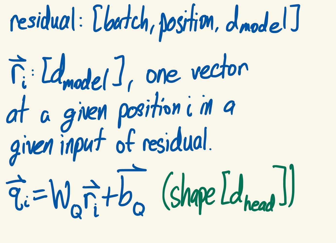
      - For a given position in a given input in the batch, there is a vector of dimension d_model in normalized_resid_pre. Call that vector r. For every r, generate one query, one key, and one value (each a vector of dimension d_head) from r:
        query = WQ(r)+bQ
        key = WK(r)+bK
        value = WV(r)+bV
      - Since we now have a vector of dimension d_head for every position and every input, the tensors for queries, keys, and values are all of shape [batch, position, d_head].
    - I will describe the next part as well as I can, but I think this video probably does a better job of it, so I highly recommend that you watch that before reading this section.
    - What computations can we perform with these queries, keys, and values that will ultimately be useful for predicting future tokens? Here’s what transformers do.
      - First, let’s look at a single query at a given position of a given input. Let’s (metaphorically) consider this query to be a question being asked from that part of the input, saying “What other parts of the input are relevant to me?”
      - Then, we look at the keys generated at all positions of that input, and consider them to be the answers given to this question.
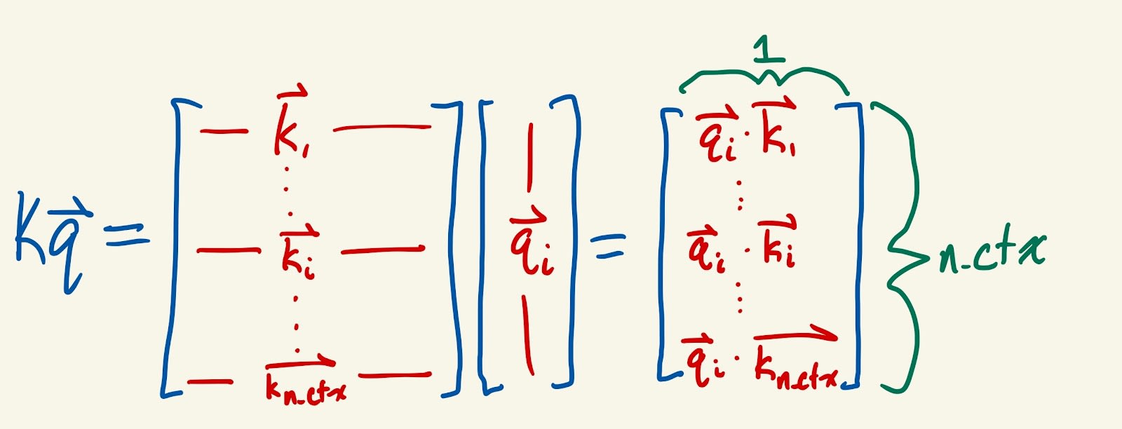
      - The better the answer is, the more attention we will direct from the query position to the key position. We measure “how good the answer is” by taking the dot product of the query with each key: call these the attention scores. The scores form a vector of dimension position (or n_ctx), since we are dotting the query with the keys of every position.
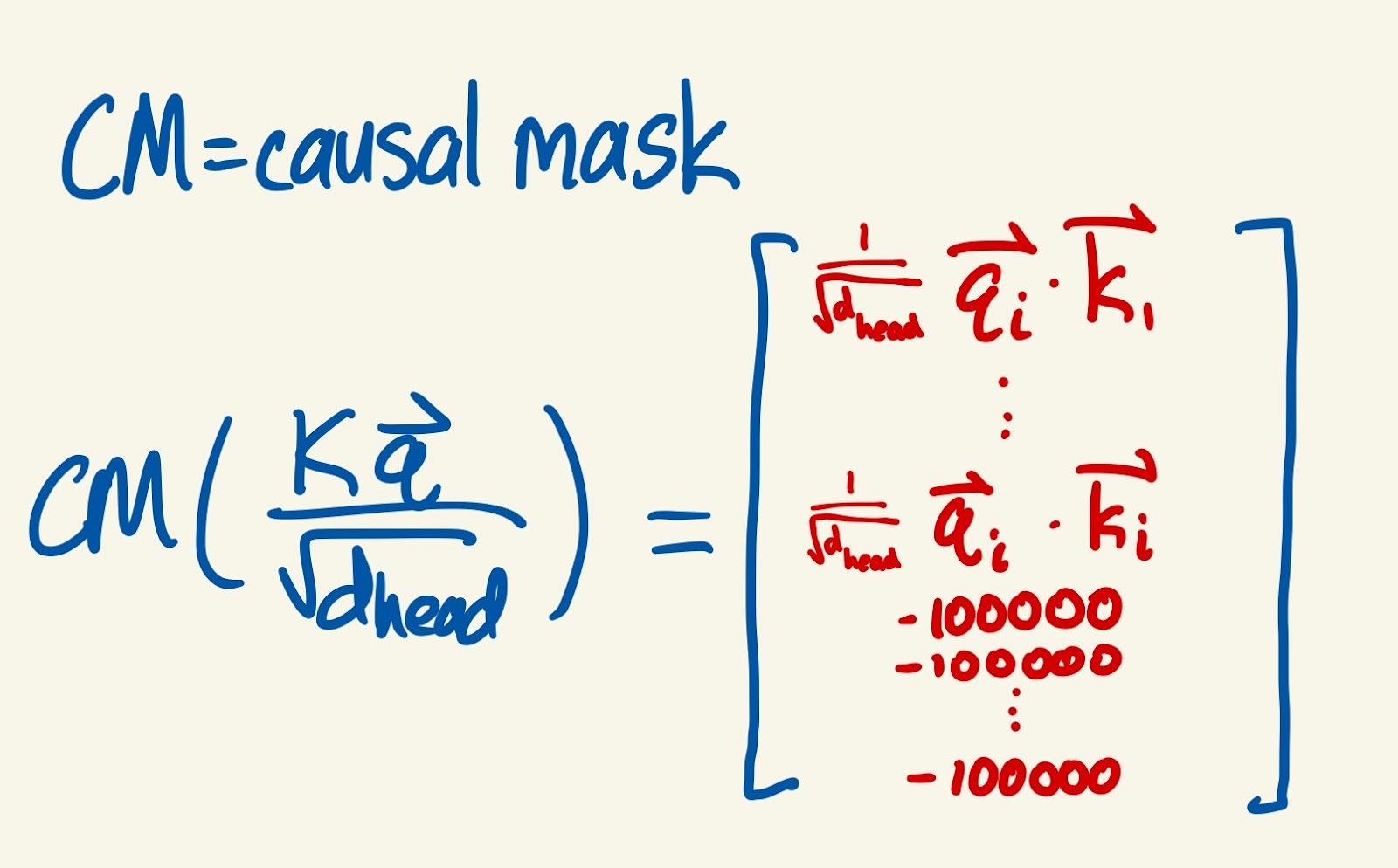
      - After that, we divide every element of this vector by $\sqrt{d_{h e a d}}$ - this step isn’t super conceptually important, it’s basically a normalization. The result is the normalized attention scores.
      - Next, we apply a causal mask to prevent the model from using any information that comes after the query position. So for every index in the normalized attention scores vector that comes after the query position, we replace the value there with a large negative number (say, -100000). The reason to use a large negative number becomes clear in the next steps, and I will also elaborate on the point of the causal mask below.
      - Then, we take the softmax of the normalized attention scores to get attention probabilities (go read about softmax if you don’t understand it!). This assigns a weight to each position of the input, such that the larger the dot product between the query and the key at a position is, the larger the weight assigned to that position is. Also, the weights add up to 1. The large negative numbers assigned by the causal mask turn into 0s after a softmax (approximately).
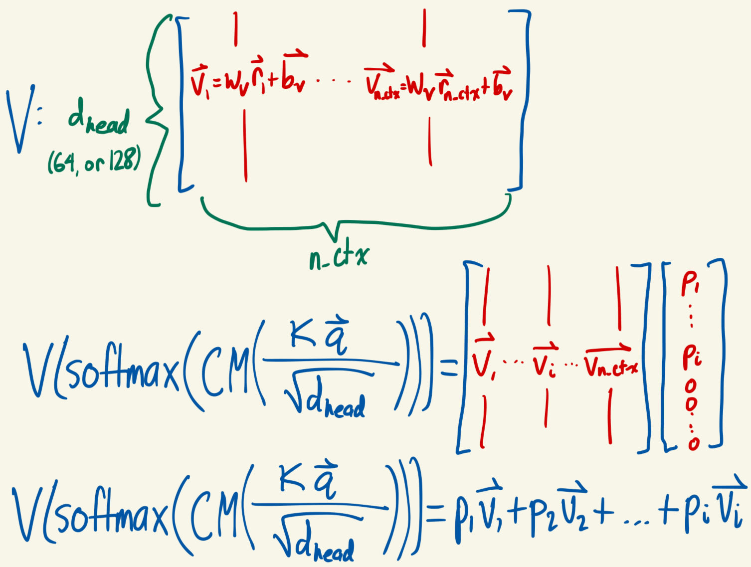
      - We use these weights to take a weighted average of the values: the larger the weight at position i, the larger the contribution of the values vector at position i to the weighted average. Since the positions after query position have weights of basically 0, the causal mask prevents any information from the input that comes after the query position from being included in the weighted average.
      - This is the point of the causal mask: the model should not be able to peek at what comes later in the sentence in order to predict what comes later in the sentence. The dimension of this weighted average vector is d_head, since each values vector has dimension d_head.
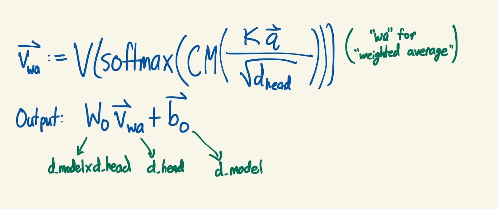
      - Finally, we use one more randomly initialized matrix; the output matrix, WO. This one has shape d_model x d_head, and maps the weighted average vector to a vector with dimension d_model. We also use one more randomly initialized bias vector, bO, also of dimension d_model, and add it to the result.
      - All of this is done for every query position in every input, so we get an output tensor of shape [batch, position, d_model].
      - Again, if this didn’t make sense, I recommend watching this video.
    - Summary of attention head: output = $(softmax (CM (\frac{Q K^{T}}{\sqrt{d_{head}}})) V) W_{O} + b_{O}$
      - Q = WQ(normalized_resid_pre)+bQ
      - This actually involves separately applying WQ to the vector at every position of the input. Same for the next two.
      - K = WK(normalized_resid_pre)+bK
      - V = WV(normalized_resid_pre)+bV
      - Shape of output: [batch, position, d_model]
      - Note: This is closer to standard notation, but looks different from what I described above in a couple of subtle ways.
        It condenses the operations for all queries, at every position of an input, into one expression. (The whole expression still needs to be done for every input in the batch.)
        The matrix multiplications are written in the opposite order: the standard matrix multiplication notation in this context is right multiplication (matrix-vector products are written as vector times matrix, 1 x a times a x b = 1 x b), but I wrote things with standard mathematical notation of left multiplication (matrix-vector products are written as matrix times vector, b x a times a x 1 = b x 1). Hopefully this adjustment isn’t too confusing - everything is conceptually the same.
  - Since there is an output for each head, the shape is currently [batch, position, d_model, n_heads]. (n_heads is the number of heads per attention layer: 12 in GPT-2, 96 in GPT-3.)
  - Sum the outputs from all attention heads. This results in shape [batch, position, d_model]. Call this tensor attn_out.
- resid_mid = residual + attn_out
- LayerNorm: Another LayerNorm exactly like the one before, but with separate learned weights and biases.
  - normalized_resid_mid = LN(resid_mid)
    - Shape: [batch, position, d_model]
- MLP: Takes normalized_resid_mid as input.
  - I’ll be very brief here since hopefully MLPs are familiar.
  - Two layers, each composed of a learned weights matrix and a learned bias vector, with one nonlinear activation function applied in the middle (GeLU is used, at least in the Neel Nanda video). The input and output layers both have dimension d_model. The hidden layer typically has dimension d_mlp = 4*d_model (though there’s no principled reason for this that I know of).
    - Hidden layer shape: [batch, position, d_mlp]
  - Call the result mlp_out.
    - Shape: You guessed it, [batch, position, d_model]
residual = resid_mid + mlp_out
- This is the output of the transformer block, also of shape [batch, position, d_model].
Remaining Transformer Blocks: GPT-3 has 96 transformer blocks. GPT-2 Small has 12. Each of them is composed of the same components as Transformer Block #1: a LayerNorm, an attention layer with attention heads, another LayerNorm, and an MLP. The input and output shape of each block is [batch, position, d_model], so the output of one block can be passed directly into the next block. This is done repeatedly until all the blocks have been completed.
- for block in blocks: residual = block(residual)
Final LayerNorm: normalized_resid_final = LN(residual)
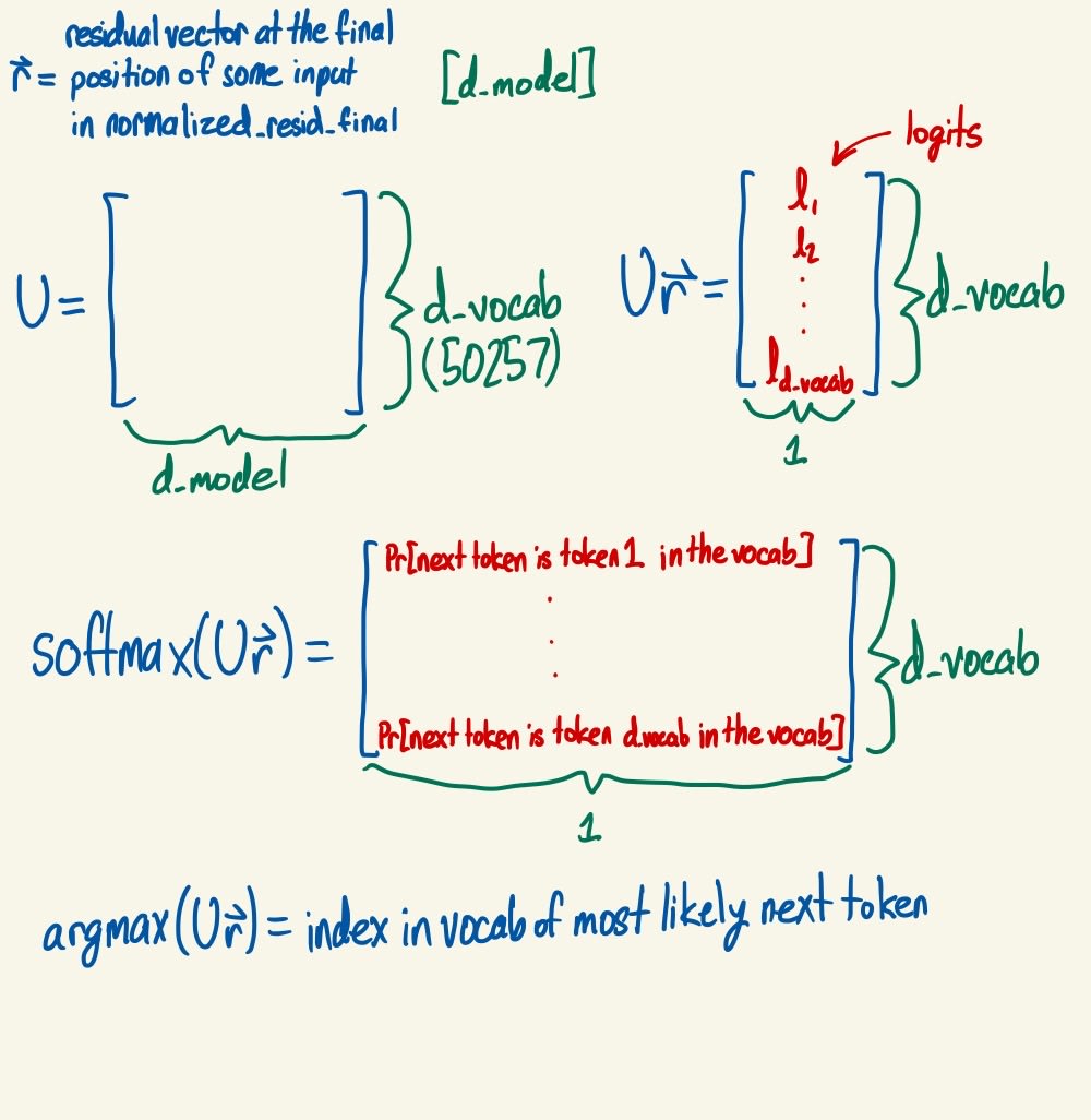
Unembed: Takes normalized_resid_final (with shape [batch, position, d_model]) as input.
- logits = Unembed(normalized_resid_final)
  - Shape: [batch, position, d_vocab]
- A d_vocab x d_model matrix is randomly initialized. This matrix multiplies the vector of dimension d_model at every position in every input to generate a logits vector of dimension d_vocab for every position in every input. Taking the softmax of the logits vector at a given position in a given input produces the probabilities that the model assigns to each token in its vocab being the token that comes after that position in the input. For the last position in any input, this produces the probabilities that the model assigns to each token in its vocab being the token that comes after the entire input.

Summary

The following is roughly the compressed understanding of transformers that I store in my head - even more compressed than the overview above.

Input: Text string. Gets converted to tokens and token indices using a prebuilt vocab.
Model:
- Embedding: Lookup table.
- Positional embedding: Add a learned value at every position and d_model component.
- A bunch of Transformer blocks: LayerNorm + Attention Layer + LayerNorm + MLP.
  - LayerNorm: Make mean 0 and variance 1, apply learned weights and biases.
  - Attention layer: A bunch of attention heads.
    - Attention heads: $(softmax (CM (\frac{Q K^{T}}{\sqrt{d_{head}}})) V) W_{O} + b_{O}$
      - Q = WQ(residual)+bQ, K = WK(residual)+bK, V = WV(residual)+bV
  - LayerNorm
  - MLP: $W_{2} (G e L U (W_{1} (r e s i d u a l)))$
- Final LayerNorm
- Unembedding: Linear map to produce logits for each token in the vocab
Output: Logits. Can be used to generate text with greedy method, or beam search, or any of several other methods.

I hope this guide was helpful!

References

0 comments

Comments sorted by top scores.

Transformers Explained (Again)

Contents

Introduction

Inputs and Outputs

Exploring Model Internals

Summary

References

0 comments