Defining Optimization in a Deeper Way Part 3
post by J Bostock (Jemist) · 2022-07-20T22:06:48.323Z · LW · GW · 0 commentsContents
  The Setup
  Example
  Further Thoughts
None
No comments
Last time I got stuck trying to remove the need for uncertainty. I have done it now! In the process I have also removed the need for absolute time.
The Setup
First we need to consider the universe as a causal network. This can be done without any notion of absolute time:
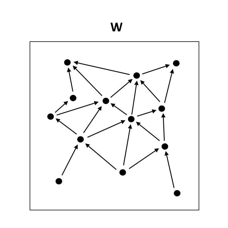
We can imagine dividing the world into two parts, and . We can represent the states of each of these parts with vectors and . We might want this division to be somewhat "natural" in the sense of John Wentworth's work on natural abstractions and natural divisions of a causal network. But it's not particularly necessary.
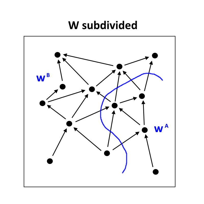
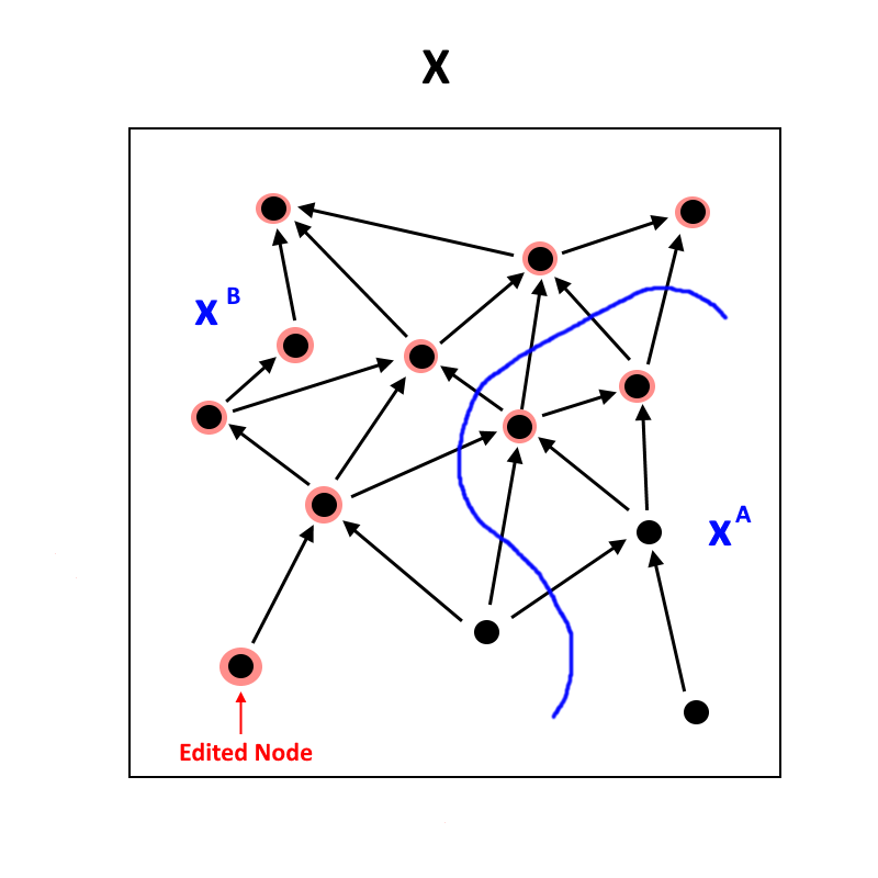
Now consider what happens if we make a small alteration to one of the variables in . Let's choose one which doesn't depend on any other variables. Everything which is "downstream" of it will be affected, so let's highlight those in red. Let's call this universe .
Now let's imagine that we take everything in , and replace it with the version from . So all of the influence coming out of will be the same as it is in . Consider what happens to . We'll call this universe , and label everything which is different from in green:
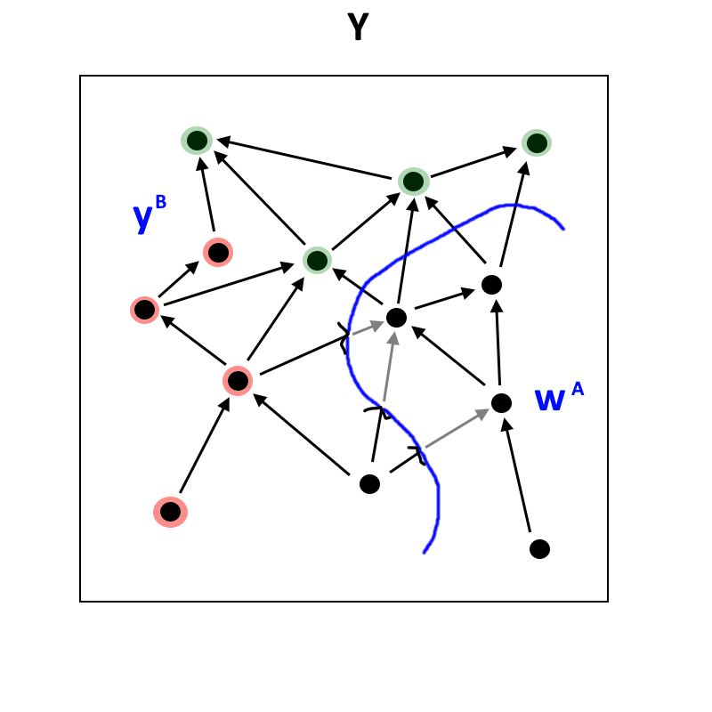
Now if any part of the universe is doing a decent job of optimizing, we would expect the influence of changing that node in to be eliminated over time. Crucially, if is optimizing , then that difference should be eliminated in , but not eliminated as much in , since has no information about the fact that is different to .
Example
Imagine our state-continuous thermostat. The causal network looks like this:
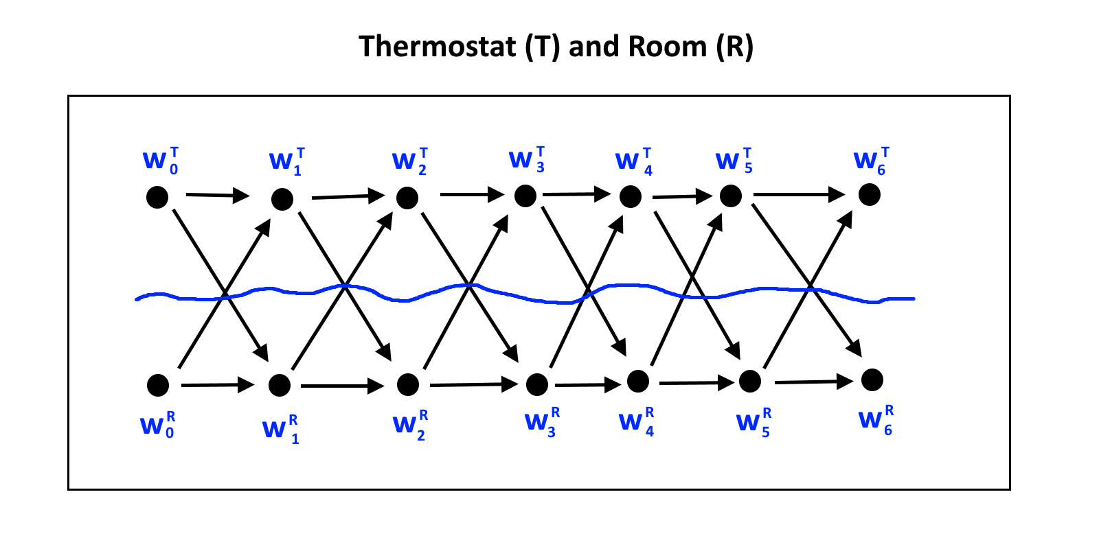
The world is divided into the thermostat and room . The dynamics of the system are described by the following equations, in which is the "desired" temperature, and represents the strength of the thermostat's ability to change the temperature of the room.
Choosing , , , and with 1000 timesteps, we can plot the course of like this:
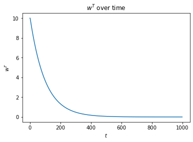
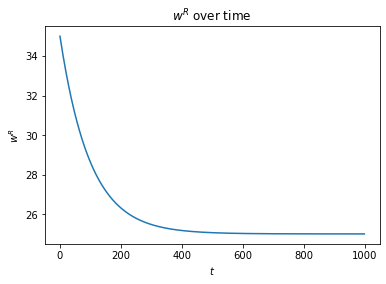
As expected, approaches 25, and approaches 25. If we choose to alter by , we can calculate , , and values. There's not much point plotting these since they're pretty much identical.
What we can plot are the relative values of and :
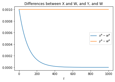
As we can see, converges to the same value as , while remains the same distance away. We can take one final measure, and plot this:
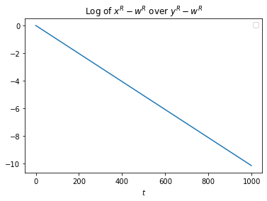
Now this plot has an interesting property in the system we are studying: it doesn't depend on our choice of .
This metric can be thought of as a sort of "compressing ability" of with respect to a change in . This optimization is measured with respect to a particular axis of variation.
The compressing ability actually doesn't change if we add some noise to the system in the form of a sinusoidal temperature variation. Even if the sinusoidal temperature variation is comically large:
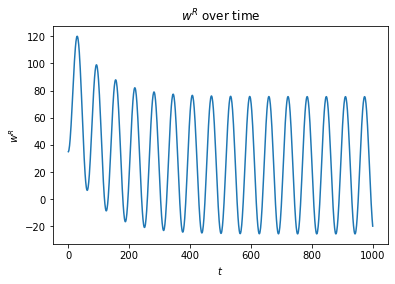

Yes, that is actually the new compressing ability being plotted, I didn't accidentally re-use the same graph! This is almost certainly a result of the fact that our "thermostat" is very mathematically pure.
What it does depend on is . With a of 0.02, we get the following:
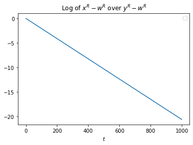
It's twice as big! This is almost too good to be true! Looks like we might actually be onto something here.
Further Thoughts
The next step is obvious. We have to measure this in systems which aren't optimizers, or are less good optimizers. If it still holds up, we can try and compare the strengths of various optimizers. Then I'd like to explore whether or not this metric is able to find optimization basins. Ideally this would involve trying to interpret some neural nets modelling some simple dynamic system.
0 comments
Comments sorted by top scores.