P=NP
post by OnePolynomial · 2024-10-17T17:56:20.635Z · LW · GW · 0 commentsContents
No comments
P = NP: Exploring Algorithms, Learning, and the Abstract Mathematical Universe
This paper presents an informal, amateur proof of P = NP, combining theoretical ideas and personal insights without the constraints of formal academic conventions.
Disclaimer: I feel completely drained from this work and just want to share it. While I can try to explain the concept, I don’t have the mental capacity for much more and plan to disengage or reduce engagement from the topic. Thank you for your understanding.
Abstract
The traditional concept of an algorithm is incomplete, as it overlooks the origin and broader context of how algorithms are created. Algorithms are developed by entities—such as AI, Turing machines, humans, animals, or other agents—interacting with the abstract/mathematical universe. We explore the idea of the abstract/mathematical universe through various real-life and pop culture examples. We discuss the impact of the process of outside learning on algorithms and their complexities. Next, we illustrate how the process of learning interacts with the abstract/mathematical universe to address the P vs NP dilemma and resolve the challenge of theoretically demonstrating the existence of polynomial algorithms, ultimately leading to the conclusion that P=NP.
The concept of abstract/mathematical universe:
This universe encompasses an infinite expanse of mathematics, concepts, and alternative universes, including imaginary physics and imaginary scenarios. For humans, it influences nearly all aspects of life: science, engineering, software, hardware, tasks, sports, entertainment, games, anime, music, art, algorithms, languages, technology, food, stories, comics and beyond. Within this universe, variables and structures like "story length" or "music genre" can be freely defined, giving rise to an overwhelming range of possibilities. For example, there are countless ways to complete an unfinished work at any point, whether it's a musical composition, a show, or something else. How many different variations of basketball or any other sport can you create? There’s an endless universe of possibilities and variables to explore.
Navigating this abstract universe without a clear direction or purpose is equivalent to solving an incomputable function. Humans and animals solve this challenge by defining finite domains, focusing only on what they need or desire within those constraints from the physical universe and the abstract universe. This principle is also the crux of AI: by creating a finite domain, AI can effectively solve problems. Interestingly, this method allows for continuous creativity—new finite domains can always be applied to generate new outcomes, such as discovering a unique drawing style. Just as there are endless video game genres and limitless card game rules, the possibilities are boundless. Practically, humans create finite domains, and AI explores them endlessly, continually discovering something new. Together, this duo enables limitless exploration and creativity.
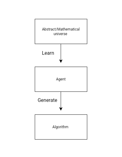
Algorithms are part of this vast abstract universe. We create them by exploring the universe, applying finite constraints, generating potential solutions, and testing them. However, the process of learning and resource consumption—which occurs outside the algorithm—is not a part of the algorithm itself. Agents such as humans, animals, or AI, acting as external explorers, can take as much time, space, and resources as necessary to traverse the abstract universe and generate new algorithms. For simplicity, we can represent such entities as Agents that operate outside the algorithm, exploring and constructing algorithms within a finite domain.
- Learning Beyond the Algorithm
Learning occurs beyond the confines of the algorithm itself. We can analyze problems or utilize AI and various techniques to explore the solution space, subsequently creating or enhancing algorithms based on those findings.
Learning is also an integral aspect of the abstract/mathematical universe, with countless methods available for acquiring knowledge. In this context, we can define learning as a mathematical process that transforms a solution space for a problem into a generalized algorithm. Theoretically, we can define agent learning as a process that can utilize time, space, and resources, as much as needed, consistently producing new and updated algorithms. This can be seen as a dynamic process that heavily impacts algorithms. Arbitrarily large learning is theoretically possible.
- Time and Space
Algorithms require both time and space, and by learning outside the algorithm, we can optimize and minimize the necessary resources. The external agent has access to as much time and resources as needed to develop a superior algorithm. It’s important to note that this improved algorithm may have a better Big O notation but could include a large number of constants. However, we can relate learning to resource usage, leading us to the following conclusions:
2.1 Time Approaches Space
This indicates that as learning increases, the time required decreases. The space mentioned here refers to input-output requirements, meaning that the theoretical limit is reached when you cannot skip the input-output processes.
Consider the evolution of multiplication algorithms: the traditional grade-school multiplication method operates in O(n²) time, where n is the number of digits. The Karatsuba algorithm reduces the time complexity to O(n^(log₂(3))) or approximately O(n^(1.585)), demonstrating how learning and improvement in algorithm design can lead to significant reductions in computational time. Further advancements, such as the Toom-Cook multiplication (also known as Toom-3), can achieve O(n^k) for some k < 1.585, and the Schönhage-Strassen algorithm, which operates in O(n log n log log n), illustrates a continued progression toward more efficient methods.
This progression highlights a pattern of reducing time complexity from O(n²) to nearly linear time, showing how learning influences algorithmic performance, and how learning optimizes time to be as close as possible to the required space, both denoted as Big O.
2.2 With More Constraints and Information, Algorithms Approach Constant Time
The addition of constraints and information can dynamically transform the efficiency of an algorithm, allowing it to approach constant time. For instance, binary search operates in logarithmic time (O(log n)) because it assumes the array is sorted. When further constraints are applied, such as knowing the precise positions of elements, we can access them directly in constant time (O(1)). This illustrates how imposing specific constraints can dramatically enhance the algorithm's efficiency, enabling it to achieve optimal performance in certain scenarios.
- Constant Space Funneling
The agent can acquire knowledge and store it within a constant amount of space. While Big O notation can sometimes be deceptive in capturing practical nuances, this concept is theoretically significant, as it can drastically reduce time complexity, bringing it closer to the input-output space. Consider this idea dynamically: after the learning process, the agent can store any necessary information as constant space to minimize time. This approach creates a powerful effect, pulling down time complexity as much as possible and tightly linking it to space.
- Human and Physical Limitations
While it's theoretically possible to utilize unlimited resources outside of the algorithm, human time is inherently limited, and physical resources are finite. To avoid spending excessive time on problems—even at the cost of some accuracy—humans develop heuristics. This is a significant reason why NP-complete problems are considered challenging; they require considerable time for analysis, making it difficult for humans to effectively observe and study exponential growth.
If we envision humans as relatively slow, they would likely create heuristics for quadratic or even linear functions. Conversely, if humans were exceptionally fast, they might more readily discover algorithms and patterns for NP-complete problems.
- Distinguishing Computability from Computational Complexity
It’s important to distinguish computability from computational complexity; they are not the same. In the context of the abstract/mathematical universe, where we theoretically have unbounded access to time, space, and resources, incomputable functions, such as the halting problem, remain unsolvable, and no algorithms can be constructed for them. In contrast, computable functions are finite and can, in theory, be learned outside the algorithm.
5.1 Growth Doesn't Matter
When operating outside the algorithm, the agent can acquire knowledge about the problem regardless of its growth rate. With the halting problem, if we are at point A, there is no possible progression to the next point B because it represents an infinite process. However, for NP-complete problems, although the growth may be substantial, it remains finite. If point A is represented by 2^6 (64) and point B by 2^7 (128), the agent can learn the necessary information and move from point A to point B outside the algorithm, effectively navigating the problem space.
It is a misconception to believe that exponential growth inherently renders a problem unsolvable or hard to solve; there exists a significant difference between theoretical complexity and practical feasibility. Exponential growth does not imply infinity; rather, it signifies a finite, albeit rapid, increase that can be addressed with the right approaches.
5.2 There Is No Need to Check All Hidden Connections
A common misconception is the belief that we must exhaustively explore all possible NP-complete assignments, theoretically. However, this assumption is incorrect, as checking every combination and hidden connection is not always necessary.
A simple counterexample illustrates this: suppose we are given an array of numbers and asked to find the sum of all possible sums of three-element pairs. The straightforward approach would involve generating a three-dimensional cube of combinations and summing all elements, resulting in a time complexity of O(n³). However, by using a more efficient multiplication-based formula, we can achieve the same result in significantly less time.
5.3 All NP-Complete Instances Have Specific Polynomial Algorithms
Additionally, there exists a polynomial algorithm for every instance of an NP-complete problem. This can be demonstrated by reverse-constructing an algorithm that targets certain areas and identifies a correct answer. If the answer is negative, we can reverse-construct an algorithm that explores only a partial area and returns a negative result. Although these algorithms are not generalized, they illustrate how each instance can be resolved without the need to exhaustively explore all possible combinations. As an example, in the case of 3SAT, if we identify which clauses are problematic and lead to contradictions, we can create a reverse-engineered algorithm that specifically targets these clauses using a constant, a mathematical process, or a variable. If we know that the instance is true, we can also develop an algorithm that checks a sample through reverse construction.
- The Process of Learning NP-Complete Problems
NP-complete problems are characterized by their exponential growth in search space. However, it’s not necessary to conduct a complete search. By applying learning and utilizing as much time and resources as needed, we can gain insights and establish connections.
For example, in the case of three-satisfiability (3-SAT), each input size has instance indexes, and each index corresponds to its own truth table. We can generate large numbers from these truth tables and identify connections and patterns, similar to how we work with lower functions and numbers. Yet, practically executing this is challenging due to human and physical limitations, as it would require dealing with trillions of large numbers, which seems unfeasible without AI or some extensive mechanism.
6.1 Ramsey Theory and Numbers
We can leverage Ramsey theory to prove the existence of patterns. According to Ramsey theory, large structures must exhibit patterns. We can use these patterns to construct a proof by induction, as there are shared patterns between an input size and the next. Observations indicate that numerous patterns exist, and the unordered nature of NP-complete problems can actually simplify our task because there is an exponential number of redundant combinations. Additionally, we know that half of these cases are merely mirrored versions of each other. Furthermore, Ramsey theory suggests that patterns can overlap, leading to a rapid increase in the number of patterns with size. By learning and having ample time and resources, discovering and utilizing these patterns in algorithms becomes inevitable. For 3SAT, despite the exponential growth, it is theoretically possible to take indexes of instances and their truth tables, create numbers from them, check the identified patterns, and construct an algorithm that solves 3SAT. We understand that these numbers are not random; they have a logical order, and there are evident patterns, as well as hidden ones.
6.2 Polynomial Bits and Polynomial Compression
To demonstrate the connection between polynomial algorithms and needed time for NP-c problems, we can observe that n bits represent 2^n possibilities. When the agent learns, it can compress its findings into polynomial space. This illustrates the power of compression: for instance, 2n bits represent twice the possibilities, allowing us to maintain a linear bit count with a constant addition, keeping it within O(n). Even higher-order functions like n! or n^n can be represented with O(n log n) bits.
Polynomial bits are sufficient for our purpose, especially in the context of NP-complete problems, as they have the capacity and expressive power to compress the search space into polynomial form. These polynomial bits can either be integrated as constant space within the algorithm or used to encode a polynomial process. We highlight the use of polynomial bits to confirm that the process remains polynomial and that the problem space can indeed be compressed into polynomial complexity.
- Summary of the Process
The process of learning and discovering polynomial algorithms for NP-complete problems can be summarized as follows:
-
The agent learns NP-complete problems: By engaging with various instances of NP-complete problems, the agent collects data and observations about their structures and properties.
-
Identifying patterns within the solution space: Utilizing insights from Ramsey theory and other mathematical frameworks, the agent identifies recurring patterns that exist across different problem instances.
-
Encoding findings using polynomial bits: The agent compresses its discoveries into polynomial bits, enabling a more efficient representation of the problem space and facilitating quicker retrieval and processing of information.
-
Constructing a polynomial algorithm for NP-complete problems: Leveraging the learned patterns and compressed information, the agent can develop an efficient polynomial algorithm that addresses specific instances of NP-complete problems.
-
Super Processing: Imagine if humans could process trillions of large numbers daily as a routine task—would NP-complete problems still be considered difficult? And what meaning would the distinction between P and NP even hold in such a scenario?
-
What is the equivalent of nondeterministic guesses? Nondeterministic guesses are simply solutions or shortcuts introduced by an agent that has learned about the problem outside the algorithm, then integrated that knowledge into it.
- Why hasn’t anyone solved P vs NP or NP-complete problems yet?
Most efforts are focused on proving the opposite.
Practical learning and solving limitations and the challenge of exponential growth.
Outdated perspectives on computation, computers, AI, and technology.
A misconception of equating computability with complexity.
- Concluding statement If agent learning can utilize as many resources as necessary, then finding polynomial algorithms for NP-complete problems becomes inevitable. Therefore, P=NP
- Conclusion We can observe how the introduction of learning processes resolves the theoretical dilemma of proving the existence of an algorithm. It also highlights that a problem's difficulty may arise from practical limitations and the sheer scale of numbers involved. This suggests the existence of another realm of polynomial algorithms, accessible only after extensive learning. It is entirely possible to have polynomial algorithms, such as O(n^2), with large constants. While this makes P = NP theoretically true but impractical, it reveals the depth of P and the many realms contained within it.
One Polynomial aka One P
0 comments
Comments sorted by top scores.