Past Tense Features

post by Can (Can Rager) · 2024-04-20T14:34:23.760Z · LW · GW · 0 comments

Contents

  TLDR
  Dataset
    Clean: While the teacher was talking, the student____
    Patch: While the teacher is talking, the student____
  Feature effects
    F(C) = L(C) – L(∅) / ( L(M) – L(∅) ).
    Destructive features (highlighted in blue)
    Recovering features
  Positional information
  Future work
None
No comments

TLDR

I find past tense features in pythia-70m using a templated dataset. My high-level steps are:

1. Creating a templated dataset that indicates past tense through a past progressive clause
2. Finding subsets of features that recover the original model performance with attribution patching
3. Analyzing the feature effects by token position

Access the code here: past_features.ipynb

Dataset

First, I define a task that elicits the model’s understanding of past tense. Given a templated prefix that indicates the tense, the model has to predict a verb in the correct form. Defining a simple template that uniquely determines the tense was tricky. I eventually chose to indicate tenses using past progressive. Here is a “clean” prefix in past progressive and its “patch” counterpart in present progressive

Clean: While the teacher was talking, the student____

Patch: While the teacher is talking, the student____

The helping verb highlighted in green uniquely determines whether the verb at the underlined position has to take a past or present form. The mean logit diff between a set of verbs in the past tense and their conjugation in present tense serves as a performance metric (measured at the final position). The performance L of the full model M on this dataset is

L(M) = sum( logits_correct_verbs ) – sum( logits_incorrect_verbs ).

The dataset contains 10 samples of clean (past) and patch (present) prefixes. For each sample I use the same set of 123 verbs to evaluate performance F. (The exact number of 123 verbs is a result of filtering a bunch of verbs that tokenize into a single token in both tenses.)

Feature effects

I investigate the SAEs trained by Sam Marks on the outputs of attention and MLP layers, and resid_post activations. In line with Sparse Feature Circuits, I fold the pretrained SAEs into the model’s computational graph and add the reconstruction error back into the forward pass. This allows me to cache feature attributions without accumulating the reconstruction error. I quantify the extent to which a set of features C recovers performance with the faithfulness score

F(C) = L(C) – L(∅) / ( L(M) – L(∅) ).

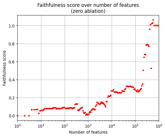
analogous to previous circuit discovery work. Here, L(C) is the model’s performance when resample-ablating all features except for the ones in set C. L(∅) is the model’s performance on all features ablated serves as a baseline. L(M) is the performance of the full model. To choose a set C, I approximate the importance of each feature using attribution patching. The patching experiment yields a ranked list of feature importances. In the plot below, I show the faithfulness for sets C containing the top n important features over a range of n.

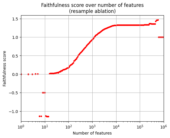
There are about 590,000 features in total. The horizontal line at faithfulness=1 for a higher number of features is included for better visibility. We can recover the original model performance with only 1000 out of 590,000 features! I expected to see the general trend between 20 and 1000 features running smoothly from 0 to 1. From about 1000 features until the final 1000 features the performance is higher than the original model performance. I suspect this arises because actively helpful features are included, while features with negative effects are ablated. The sudden dips around 10 nodes are unexpected. Zooming in shows that two features in MLP0 (highlighted in blue) cause these dips.

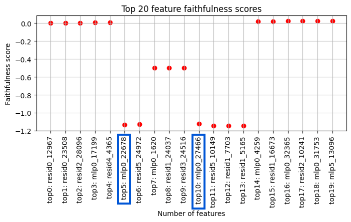
Note, that I perform resample-ablation. Each point represents that the corresponding feature and features with a higher effect see the clean helping verb “ was” while all features with a lower effect see the patch helping verb “ is”. The two “destructive features” highlighted in blue significantly lower faithfulness to a regime where the model is more likely to predict the patch answer. Interestingly, this effect is fully canceled out by the “recovering features” mlp0_1620 and mlp0_4259 in the same layer. Using Neuronpedia, I annotated on which those features activate.

Destructive features (highlighted in blue)

mlp0_22678: “ was”

mlp0_22466: “ is”, but with light activations on all forms of to be even abbreviations like “‘s”.

Recovering features

mlp0_1620: “ was”

mlp_4259: “ is”

The corresponding destructive and recovering features activate on the same tokens. My first guess is that the corresponding features are highly correlated. I leave the correlation analysis or future work. The Neuronpedia dashboards for all four features look quantitatively similar, here’s an example for the final negative feature.

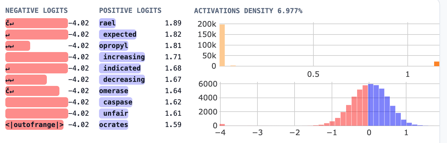
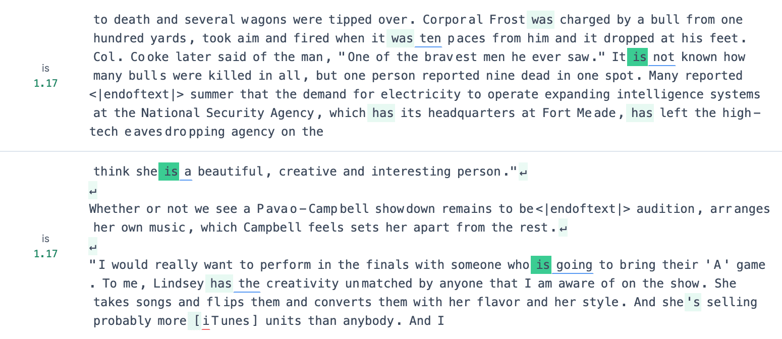
The top activating examples and the significant gap in the activations density plot suggest that these features are specific token detectors. At this early position in the model, specific token detectors act as an additional embedding. Similar experiments with GPT2-small, showed that the MLP0 layer often serves as an extension of the embedding.

The early dips in faithfulness are an artifact of the resample ablation. They don’t occur when I run the faithfulness experiment with zero-ablation. The minimum faithfulness score for zero-ablation is 0, as expected. In my opinion, using resample-ablation is more principled: With zero-ablation, the model internals are perturbed too heavily and the faithfulness trajectory is way messier.

Positional information

Finally, feature effects indicate how information is moved between positions. The plot below shows the mean feature activations per position for each SAE.

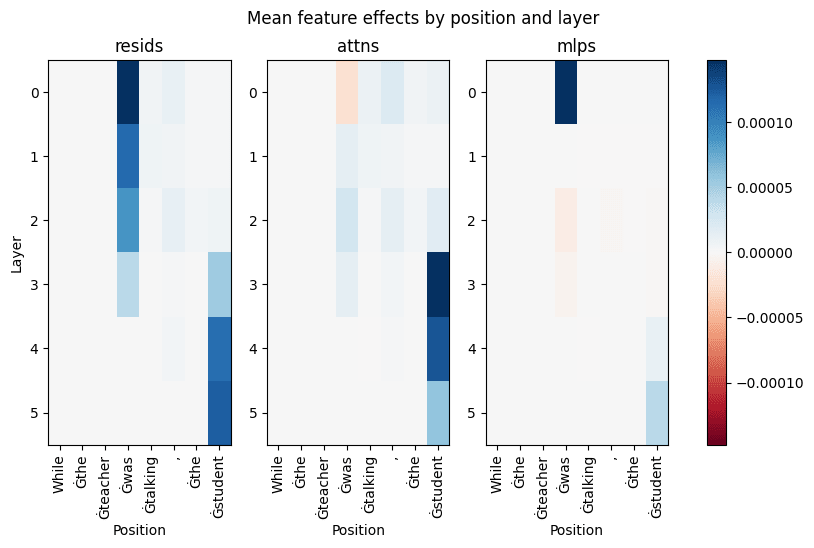
In the early layers of the residual stream, the most important features are clearly firing on the position of the helping verb. In layer 3, attention heads move the information of the tense to the final position. I suspect this is the point at which the model realizes that the next token has to be a verb and starts collecting relevant information at the final position. The attention layers further show slight mean effects at the helping verb and comma positions. Note, that we are looking at the mean effect across all 32768 features in each layer. There could be a small amount of highly active features in the early attention layers, whose effect is not clearly visible due to many inactive features in the same layer. MLP0 has a significant feature effect at the helping verb position, which supports the hypothesis that this layer acts as an embedding. To sum it up, the Figure clearly shows how the information of the past tense is being moved from the helping verb in the first clause to the final position.

Future work

As a concrete next step, I would like to analyze the structure of attention heads in early layers. Further, a correlation analysis for the destructive and recovering features would be useful to track down the cause of the dips in the faithfulness plot. Moreover, I could run the experiment on a more complex prompt. When I initially designed the dataset, I wanted to elicit the capability of “identifying the past progressive tense in the first clause and deducing that the second clause has to be in the past.” However, I investigated a prompt simpler than that. The correct prediction of a verb in past tense in the second clause can simply be solved with the heuristic “I detect the token ‘ was’ so all following verbs must be in past tense”. This simple heuristic can be avoided by making the template more complex. For example, I could plug a relative clause in present tense between the first and second clause.  Finally, an analogous experiment can be done for features in the present tense!

0 comments

Comments sorted by top scores.