Grue, Bleen, and natural categories
post by Stuart_Armstrong · 2015-07-06T13:47:26.487Z · LW · GW · Legacy · 0 commentsContents
  Natural category, probability flows
  Less pictures, more math
  Almost natural category
  Beyond boolean
  And in practice?
None
No comments
A putative new idea for AI control; index here.
In a previous post, I looked at unnatural concepts such as grue (green if X was true, blue if it was false) and bleen. This was to enable one to construct the natural categories that extend AI behaviour, something that seemed surprisingly difficult to do.
The basic idea discussed in the grue post was that the naturalness of grue and bleen seemed dependent on features of our universe - mostly, that it was easy to tell whether an object was "currently green" without knowing what time it was, but we could not know whether the object was "currently grue" without knowing the time.
So the naturalness of the category depended on the type of evidence we expected to find. Furthermore, it seemed easier to discuss whether a category is natural "given X", rather than whether that category is natural in general. However, we know the relevant X in the AI problems considered so far, so this is not a problem.
Natural category, probability flows
Fix a boolean random variable X, and assume we want to check whether the boolean random variable Z is a natural category, given X.
If Z is natural (for instance, it could be the colour of an object, while X might be the brightness), then we expect to uncover two types of evidence:
- those that change our estimate of X; this causes probability to "flow" as follows (or in the opposite directions):
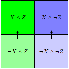
- ...and those that change our estimate of Z:
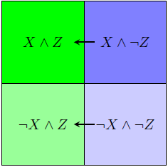
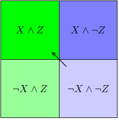
Or we might discover something that changes our estimates of X and Z simultaneously. If the probability flows to X and and Z in the same proportions, we might get:
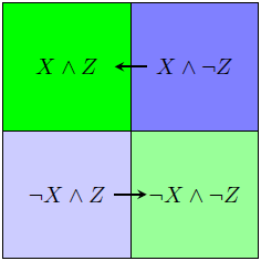
What is an example of an unnatural category? Well, if Z is some sort of grue/bleen-like object given X, then we can have Z = X XOR Z', for Z' actually a natural category. This sets up the following probability flows, which we would not want to see:
More generally, Z might be constructed so that X∧Z, X∧¬Z, ¬X∧Z and ¬X∧¬Z are completely distinct categories; in that case, there are more forbidden probability flows:
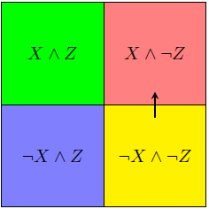
and
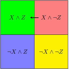
In fact, there are only really three "linearly independent" probability flows, as we shall see.
Less pictures, more math
Let's represent the four possible state of affairs by four weights (not probabilities):
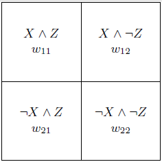
Since everything is easier when it's linear, let's set w11 = log(P(X∧Z)) and similarly for the other weights (we neglect cases where some events have zero probability). Weights are correspond to the same probabilities iff you get from one set to another by multiplying by a strictly positive number. For logarithms, this corresponds to adding the same constant to all the log-weights. So we can normalise our log-weights (select a single set of representative log-weights for each possible probability sets) by choosing the w such that
w11 + w12 + w21 + w22 = 0.
Thus the probability "flows" correspond to adding together two such normalised 2x2 matrices, one for the prior and one for the update. Composing two flows means adding two change matrices to the prior.
Four variables, one constraint: the set of possible log-weights is three dimensional. We know we have two allowable probability flows, given naturalness: those caused by changes to P(X), independent of P(Z), and vice versa. Thus we are looking for a single extra constraint to keep Z natural given X.
A little thought reveals that we want to keep constant the quantity:
w11 + w22 - w12 - w21.
This preserves all the allowed probability flows and rules out all the forbidden ones. Translating this back to a the general case, let "e" be the evidence we find. Then if Z is a natural category given X and the evidence e, the following quantity is the same for all possible values of e:
log[P(X∧Z|e)*P(¬X∧¬Z|e) / P(X∧¬Z|e)*P(¬X∧Z|e)].
If E is a random variable representing the possible values of e, this means that we want
log[P(X∧Z|E)*P(¬X∧¬Z|E) / P(X∧¬Z|E)*P(¬X∧Z|E)]
to be constant, or, equivalently, seeing the posterior probabilities as random variables dependent on E:
- Variance{log[ P(X∧Z|E)*P(¬X∧¬Z|E) / P(X∧¬Z|E)*P(¬X∧Z|E) ]} = 0.
Call that variance the XE-naturalness measure. If it is zero, then Z defines a XE-natural category. Note that this does not imply that Z and X are independent, or independent conditional on E. Just that they are, in some sense, "equally (in)dependent whatever E is".
Almost natural category
The advantage of that last formulation becomes visible when we consider that the evidence which we uncover is not, in the real world, going to perfectly mark Z as natural, given X. To return to the grue example, though most evidence we uncover about an object is going to be the colour or the time rather than some weird combination, there is going to be somebody who will write things like "either the object is green, and the sun has not yet set in the west; or instead perchance, those two statements are both alike in falsity". Upon reading that evidence, if we believe it in the slightest, the variance can no longer be zero.
Thus we cannot expect that the above XE-naturalness be perfectly zero, but we can demand that it be low. How low? There seems no principled way of deciding this, but we can make one attempt: that we cannot lower it be decomposing Z.
What do we mean by that? Well, assume that Z is a natural category, given X and the expected evidence, but Z' is not. Then we can define a new category boolean Y to be Z with high probability, and Z' otherwise. This will still have low XE-naturalness measure (as Z does) but is obviously not ideal.
Reversing this idea, we say Z defines a "XE-almost natural category" if there is no "more XE-natural" category that extends X∧Z (and the other for conjunctions). Technically, if
X∧Z = X∧Y,
Then Y must have equal or greater XE-naturalness measure to Z. And similarly for X∧¬Z, ¬X∧Z, and ¬X∧¬Z.
Note: I am somewhat unsure about this last definition; the concept I want to capture is clear (Z is not the combination of more XE-natural subvariables), but I'm not certain the definition does it.
Beyond boolean
What if Z takes n values, rather than being a boolean? This can be treated simply.
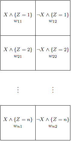
If we set the wjk to be log-weights as before, there are 2n free variables. The normalisation constraint is that they all sum to a constant. The "permissible" probability flows are given by flows from X to ¬X (adding a constant to the first column, subtracting it from the second) and pure changes in Z (adding constants to various rows, summing to 0). There are 1+ (n-1) linearly independent ways of doing this.
Therefore we are looking for 2n-1 -(1+(n-1))=n-1 independent constraints to forbid non-natural updating of X and Z. One basis set for these constraints could be to keep constant the values of
wj1 + w(j+1)2 - wj2 - w(j+1)1,
where j ranges between 1 and n-1.
This translates to variance constraints of the type:
- Variance{log[ P(X∧{Z=j}|E)*P(¬X∧{Z=j+1}|E) / P(X∧{Z=j+1}|E)*P(¬X∧{Z=j}|E) ]} = 0.
But those are n different possible variances. What is the best global measure of XE-naturalness? It seems it could simply be
- Max_jk Variance{log[ P(X∧{Z=j}|E)*P(¬X∧{Z=k}|E) / P(X∧{Z=k}|E)*P(¬X∧{Z=j}|E) ]} = 0.
If this quantity is zero, it naturally sends all variances to zero, and, when not zero, is a good candidate for the degree of XE-naturalness of Z.
The extension to the case where X takes multiple values is straightforward:
- Max_jklm Variance{log[ P({X=l}∧{Z=j}|E)*P({X=m}∧{Z=k}|E) / P({X=l}∧{Z=k}|E)*P({X=m}∧{Z=j}|E) ]} = 0.
Note: if ever we need to compare the XE-naturalness of random variables taking different numbers of values, it may become necessary to divide these quantities by the number of variables involved, or maybe substitute a more complicated expression that contains all the different possible variances, rather than simply the maximum.
And in practice?
In the next post, I'll look at using this in practice for an AI, to evade presidential deaths and deflect asteroids.
0 comments
Comments sorted by top scores.