AI could cause a drop in GDP, even if markets are competitive and efficient

post by Casey Barkan (casey-barkan) · 2025-04-10T22:35:16.290Z · LW · GW · 0 comments

Contents

  Model
    Solving the model for a choice of parameters
None
No comments

I present a macroeconomic model of a competitive economy that, counterintuitively, predicts that increases in the productivity of automation technology will decrease economic production. In the model, the decrease in production occurs over an intermediate range of automation productivities, and once automation productivity is high enough that all labor is replaced, production begins to rise.

Most discussions of the economic impacts of AI assume that automation will increase total economic output. Even though wages may decline, the common assumption is that total production will rise. However, in this post I show that a basic model that follows a standard macroeconomic modeling framework predicts otherwise. The model starts with a simple general equilibrium model of a competitive economy and incorporates an automation technology whose productivity increases over time. This model predicts that the increasing productivity of automation causes GDP to decline until all production is automated, at which point GDP begins to rise again and eventually surpasses its pre-automation level. Even a temporary decline in GDP could cause lasting effects: for example, falling tax revenue could destabilize governments, undermining universal basic income (UBI) and AI safety policies.

The mechanism responsible for the drop in GDP is that automation causes wages to fall, and as they fall the amount of labor that workers provide also falls. The drop in labor causes a drop in production that can be greater than the increase in production due to higher productivity automation. To my knowledge, this conceptual argument was first proposed by Artūrs Kaņepājs^[1]. Later, I developed a model showing that AI can decrease GDP in a non-competitive economy^[2][3]. It turns out that a drop in GDP can occur even in a competitive economy with frictionless markets, as shown in this post.

The model is defined and solved in the section below, and Figure 1 shows the equilibrium quantities as a function of $A_{\text{auto}}$, the productivity of automation technology. Note that I used the simplest (not the most realistic) choice of parameters to make the figure. The economy's output (left panel, blue curve) drops sharply when $A_{\text{auto}}$ surpasses the threshold $R_0$, and falls until labor employed is zero, at which point output begins to rise. At low $A_{\text{auto}}$, returns to labor and capital are equal, but at high $A_{\text{auto}}$ all output goes to capital owners.

Is Figure 1 a quantitative prediction of what will happen in the real world? Certainly not, both because the model is very simplistic and because I made no attempt to choose realistic parameters when plotting the figure. One adjustment to the parameters can be made to make the prediction a bit more plausible: setting parameters so that pre-automation labor supplied is half of the maximum labor that humans could supply^[4] yields a drop in GDP of 8%. This is smaller than the drop shown in Figure 1, but still twice as large as the drop in U.S. GDP during the 2008 recession.

Model

The model is a standard general equilibrium model with a production function that incorporates AI automation. I'm interested in extending the model to make it more realistic, and I'm very interested in hearing opinions about which assumptions or missing features of the model are in most need of improvement.

Production: There are an unspecified^[5] number of firms with access to the same production function and which compete with one another. The production function is determined by two available technologies: the old technology (described by a Cobb-Douglas production function) which requires capital^[6] $K$ and labor $L$ to be utilized together, and an automation technology (described by an AK production function) which allows production without labor input. The production functions for these technologies are $f_{\text{old}}(K,L)=A_{\text{old}}{K}^{\alpha }{L}^{1-\alpha }$ with $0<\alpha <1$, and $f_{\text{auto}}\left(K\right)=A_{\text{auto}}K$. The productivity of AI automation, $A_{\text{auto}}$, is assumed to be zero initially and increases as AI technology improves, and we will compute the equilibrium as a function of $A_{\text{auto}}$^[7]. The total production function is determined by allocating capital between the two technologies so as to maximize output for the given inputs:

$$F(K,L)=\underset{0\le K_{\text{old}}\le K}{max}\left\{f_{\text{old}}(K_{\text{old}},L)+f_{\text{auto}}(K-K_{\text{old}})\right\}$$

The $K_{\text{old}}$ that solves this maximization problem is

$$K_{\text{old}}=\{\begin{array}{cc}K& A_{\text{auto}}<\alpha A_{\text{old}}(L/K{)}^{1-\alpha }\\ {\left(\frac{\alpha A_{\text{old}}}{A_{\text{auto}}}\right)}^{\frac{1}{1-\alpha }}L& A_{\text{auto}}\ge \alpha A_{\text{old}}(L/K{)}^{1-\alpha }\end{array}$$

so the production function simplifies to

$F(K,L)=\{\begin{array}{cc}{A}_{\text{old}}{K}^{\alpha }{L}^{1-\alpha }& A_{\text{auto}}<\alpha A_{\text{old}}(L/K{)}^{1-\alpha }\\ ({\alpha }^{\frac{\alpha }{1-\alpha }}-{\alpha }^{\frac{1}{1-\alpha }})\frac{A_{\text{old}}^{\frac{1}{1-\alpha }}}{A_{\text{auto}}^{\frac{\alpha }{1-\alpha }}}L+A_{\text{auto}}K& A_{\text{auto}}\ge \alpha A_{\text{old}}(L/K{)}^{1-\alpha }\end{array}$

Notice that for low $A_{\text{auto}}$, capital and labor are complements, but once $A_{\text{auto}}$ surpasses a threshold, capital and labor become perfect substitutes.

Capital supply: A fixed capital stock $K$ is assumed. Of course, savings lets capital accumulate over time, so this assumption precludes using the model to study long-run growth.

Labor supply: Labor supplied is a function of wage $W$, denoted $L^s\left(W\right)$. I assume there is a reservation wage $W_R$ below which zero labor is supplied. There are a few reasons why we should expect a reservation wage:

• If wages drop so low that workers can no longer subsist, then labor supplied will drop to zero.
• Labor supplied could fall very low even before wages drop to subsistence levels if wages are low enough that workers prefer to live off of their savings or government welfare.
• A minimum wage may legally enforce that no labor is employed at wages below a set minimum.

The labor supply can be microfounded by assuming that households select $L^s\left(W\right)$ by maximizing a utility function, as is done in the example below. Note that I assume $L^s\left(W\right)$ is independent of $R$, the rental rate of capital, which is to assume that laborers own no capital.

Competitive markets: Labor and capital are paid their marginal products, i.e. $W=F_L(K,L)$ and $R=F_K(K,L)$^[8], as is the case in competitive markets^[9].

Computing the equilibrium: With the market clearing condition $L=L^s\left(W\right)$, we have $W=F_L(K,L^s(W\left)\right)$ which can be solved to obtain $W$, which in turn determines $L$. Inserting $K$ and $L$ into the production function yields total output, and rental rate is given by $R=F_K(K,L)$.

The three regimes of production: The equilibrium production can be written in a way that reveals the three regimes (for low, intermediate, and high $A_{\text{auto}}$) that are apparent in Figure 1. At low $A_{\text{auto}}$, automation technology is completely unutilized. Once $A_{\text{auto}}$ surpasses the threshold $\alpha A_{\text{old}}(L/K{)}^{1-\alpha }$ automation begins to be utilized. Note that this threshold is equal to rental rate $R=F_K(K,L)$. As $A_{\text{auto}}$ continues to rise, wages drop until reaching the reservation wage $W_R$; denote the value of $A_{\text{auto}}$ where this occurs as $A_{\text{Displace}}$. Above $A_{\text{Displace}}$, $L=0$ and $K_{\text{old}}=0$. Letting $L_0$ and $R_0$ denote the equilibrium labor and rental rate when $A_{\text{auto}}=0$, the equilibrium production $F_{\text{Eq}}\left(A_{\text{auto}}\right)$ can now be written as

$F_{\text{Eq}}\left(A_{\text{auto}}\right)=\{\begin{array}{cc}{A}_{\text{old}}{K}^{\alpha }{L}_0^{1-\alpha }& A_{\text{auto}}<R_0\\ ({\alpha }^{\frac{\alpha }{1-\alpha }}-{\alpha }^{\frac{1}{1-\alpha }})\frac{A_{\text{old}}^{\frac{1}{1-\alpha }}}{A_{\text{auto}}^{\frac{\alpha }{1-\alpha }}}{L}_{\text{Eq}}\left(A_{\text{auto}}\right)+A_{\text{auto}}K& R_0\le A_{\text{auto}}<A_{\text{Displace}}\\ A_{\text{auto}}K& A_{\text{auto}}\ge A_{\text{Displace}}\end{array}$

Solving the model for a choice of parameters

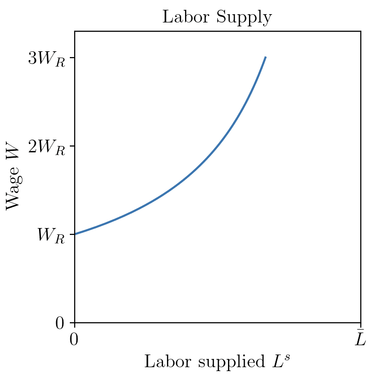
I will set $\alpha =\frac{1}{2}$ and assume $L^s\left(W\right)=\overline{L}(1-\frac{W_R}{W})$ for $W>W_R$ and $L^s\left(W\right)=0$ for $W\le W_R$ ^[10]. This labor supply curve is shown in Figure 2, and note that it has a reservation wage of $W_R$ and has a maximum labor supplied of $\overline{L}$ in the limit that wage tends to infinity. It will be convenient to rewrite the labor supply as $W=W_R/(1-L^s/\overline{L})$. This labor supply curve can be derived from a representative household with utility $u(C,L)=(2\overline{L}{W}_R+C)(2\overline{L}-L)$.

For $A_{\text{auto}}<R_0$, where $L=L_0$, we have $W=W_R/(1-L_0/\overline{L})=F_L(K,L_0)=\frac{A_{\text{old}}\sqrt{K}}{2\sqrt{L_0}}$. Solving for $L_0$ yields

$$L_0=\overline{L}-\frac{1}{2\gamma }(\sqrt{1+4\gamma \overline{L}}-1)$$

where $\gamma ={\left(\frac{A_{\text{old}}}{2W_R\overline{L}}\right)}^{2}K$. Rental rate $R_0=F_K(K,L_0)=\frac{1}{2}{A}_{\text{old}}\sqrt{\frac{L_0}{K}}$.

For $A_{\text{auto}}>R_0$, the production function greatly simplifies (thanks to the choice $\alpha =\frac{1}{2}$) to $F(K,L)=\frac{A_{\text{old}}^2}{4A_{\text{auto}}}L+A_{\text{auto}}K$. Setting $W=F_W(K,L)=W_R/(1-L/\overline{L})=F_L(K,L)$ and solving for $L$ yields the equilibrium labor, $L_{\text{Eq}}\left(A_{\text{auto}}\right)=\overline{L}(1-\frac{4W_R{A}_{\text{auto}}}{A_{\text{old}}^2})$. Note that $R=A_{\text{auto}}$ and $W=\frac{A_{\text{old}}^2}{4A_{\text{auto}}}$ in this regime, meaning rents are increasing, wages are decreasing, and labor is decreasing as automation technology improves.

$A_{\text{Displace}}$, the value of $A_{\text{auto}}$ where labor is fully displaced, can now be found. Setting $L_{\text{Eq}}\left(A_{\text{Displace}}\right)=0$ yields $A_{\text{Displace}}=\frac{A_{\text{old}}^2}{4W_R}$.

Equilibrium production can now be written as 

$F_{\text{Eq}}\left(A_{\text{auto}}\right)=\{\begin{array}{cc}{A}_{\text{old}}{K}^{\alpha }{L}_0^{1-\alpha }& A_{\text{auto}}<R_0\\ \overline{L}(\frac{A_{\text{old}}^2}{4A_{\text{auto}}}-W_R)+A_{\text{auto}}K& R_0\le A_{\text{auto}}<A_{\text{Displace}}\\ A_{\text{auto}}K& A_{\text{auto}}\ge A_{\text{Displace}}\end{array}$

To generate Figure 1, I used $A_{\text{old}}=1$, $K=1$, $W_R=1$, and $\overline{L}=1$.

1. ^{^}

   Kaņepājs, Beware Profit-Driven Automation that Shrinks the Economy, EA Forum, Oct 5 2023 (link [EA · GW])

2. ^{^}

   Barkan, Can an increase in productivity cause a decrease in production? Insights from a model economy with AI automation, ArXiv, Nov 24 2024 (link)

3. ^{^}

   At the time, I thought that a market inefficiency, such as lack of competition, was required to get a decrease in GDP. But this turns out not to be the case. 

4. ^{^}

   This comes from estimating that a 40 hour work week is roughly half of the maximum that humans could work.

5. ^{^}

   As is typical of general equilibrium models, the number of firms has no effect on the model's predictions because the production function is constant returns to scale in the factors $K$ and $L$.

6. ^{^}

   In economics, capital refers to the physical machinery used in production, which includes compute resources. This model does not differentiate between different forms of capital, which is a common simplification (see this and this), but clearly not realistic.

7. ^{^}

   One could model how the equilibrium changes in time by introducing dynamics for $A_{\text{auto}}$ into the model, as would be done in an endogenous growth model.

8. ^{^}

   The subscripts denote derivatives with respect to the given variable.

9. ^{^}

   Because $F(K,L)$ is constant returns to scale, this condition on $W$ and $R$ ensures firms' profits are zero, as is the case in competitive equilibrium.

10. ^{^}

    These choices were made solely to keep the equations simple while still adhering to the conditions for labor supply stated above.

0 comments

Comments sorted by top scores.