The Geometry of Linear Regression versus PCA

post by criticalpoints · 2025-02-23T21:01:33.415Z · LW · GW · 2 comments

This is a link post for https://eregis.github.io/blog/2025/02/23/geometry-pca-regression.html

Contents

2 comments

In statistics, there are two common ways to "find the best linear approximation to data": linear regression and principal component analysis. However, they are quite different---having distinct assumptions, use cases, and geometric properties. I remained subtly confused about the difference between them until last year. Although what I'm about to explain is standard knowledge in statistics, and I've even found well-written blog posts on this exact subject, it still seems worthwhile to examine, in detail, how linear regression and principal component analysis differ.

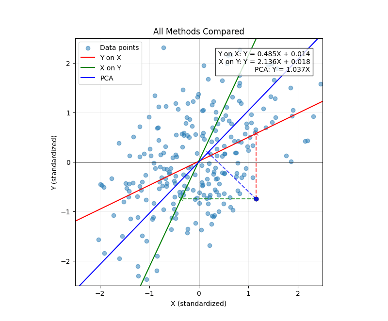
The brief summary of this post is that the different lines result from the different directions in which we minimize error:

• When we regress $Y$onto $X$, we minimize vertical errors relative to the line of best fit.
• When we regress $X$ onto $Y$, we minimize horizontal errors relative to the line of best fit.
• When we plot the first principal component of $X$ and $Y$, we minimize orthogonal errors relative to the line of best fit.

To understand the difference, let's consider the joint distribution of heights for father-son pairs where both are adults. When you observe the distribution of heights among adult men, you'll notice two key things.

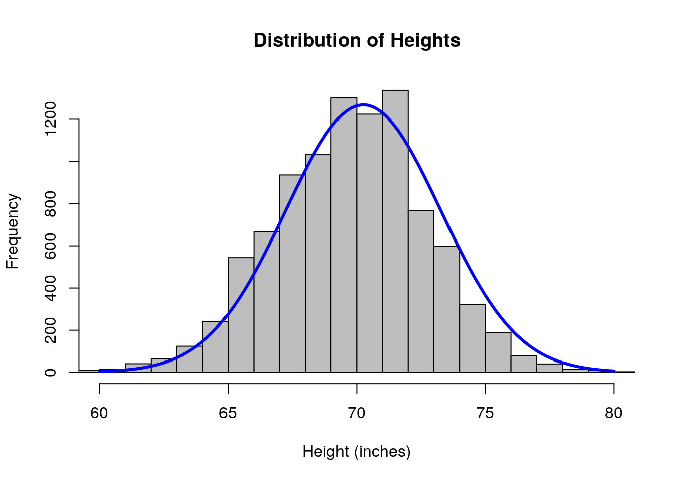
First, height in adult men is roughly normally-distributed. While some people are taller or shorter than average, there aren't 10ft tall people or 1ft tall people. The vast majority of adult men are somewhere between 5 feet and 7 feet tall. If you were to randomly sample adult males in the US and plot the data, it would form a bell-curve shaped graph like this one:

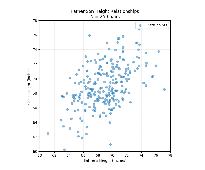
Second, height runs in families. While there is natural variation, people with taller parents tend to be taller than average. Quantitatively, the correlation between father-son height is around 0.5 (the exact value won't matter for this post).

We can create simulated data that would resemble the actual distribution of father-son heights. We'll make the following assumptions:

1. Since we are only considering adult men, we'll assume the marginal distributions of fathers and sons are exactly the same. In reality, this wouldn't be quite true for various reasons (e.g., nutrition has changed over time), but it's close enough to true, and assuming this symmetry will help make certain conceptual points clearer.
2. Both fathers and sons are normally distributed with a mean of 69 inches (5 foot 9 inches) and a standard deviation of three inches.
3. The correlation between father and son heights is 0.5. Without delving into the math, this is straightforward to simulate because everything here is Gaussian: both variables are Gaussian and the independent error term is Gaussian. Since the sum of Gaussian random variables is another Gaussian random variable, it was simply a matter of tuning the error strength to get the desired correlation.

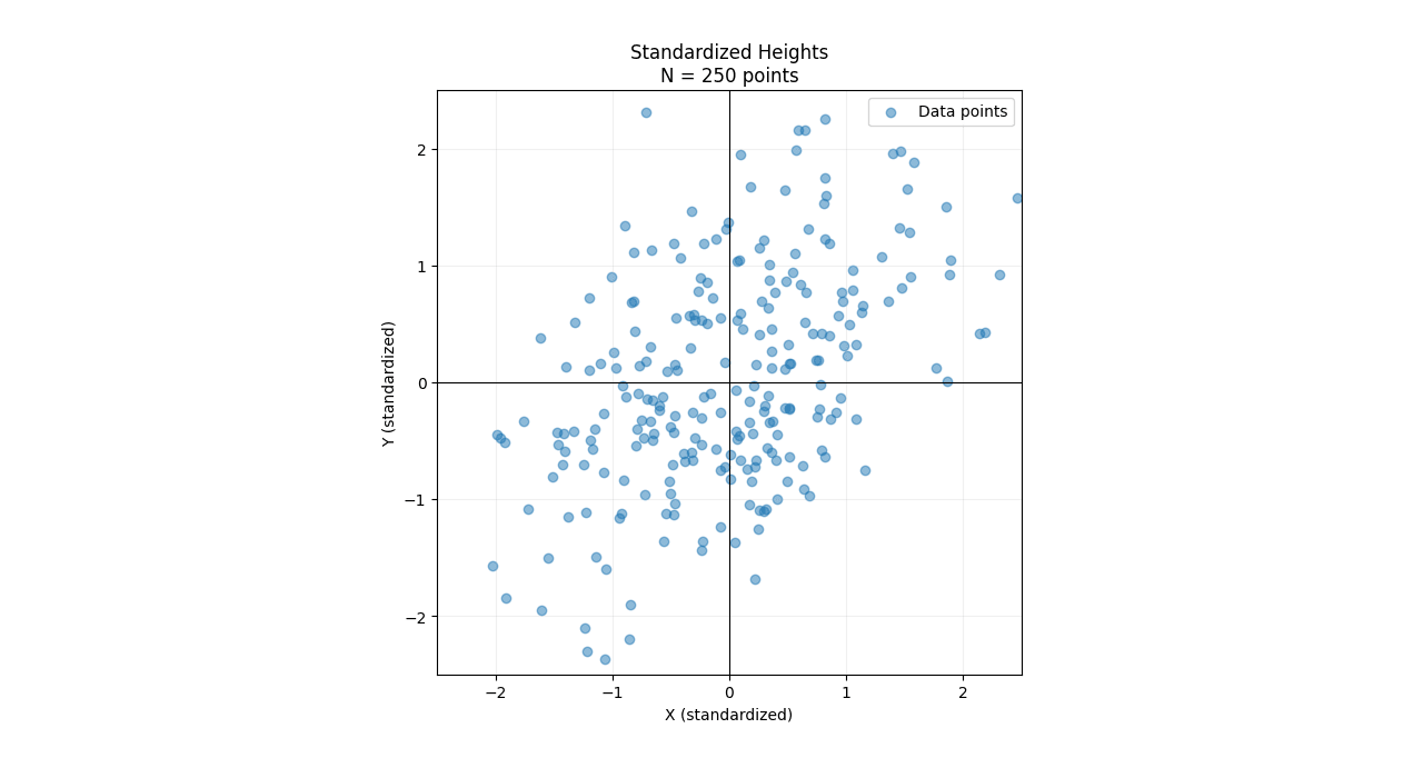
Before performing linear regression and principal component analysis, it helps to standardize the data. This involves: (1) centering the data so both distributions have a mean of zero, and (2) scaling the data so their variance equals 1. This transformation maps both distributions to standard Gaussians. Although we are transforming the data to make it easier to interpret, we preserve the 0.5 correlation between the two distributions. We will let $X$ be the standardized Gaussian random variable corresponding to the height of the father and $Y$ be the standardized Gaussian random variable corresponding to the height of the son.

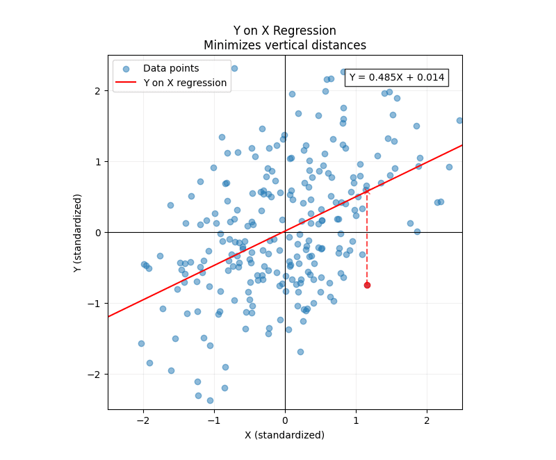
First, let's start with linear regression. When you regress $Y$ onto $X$, you are attempting to answer the question: "Given a value of $X$, what is our best guess at the value of $Y$"? In our example, this means: "Given the height of the father, what is our best guess at the height of the son?"

"Best guess" is determined by the cost function. For linear regression, the cost function is the least-squares:

$$J_Y\left({\beta }_Y\right)=|Y-{\beta }_{Y}X{|}^2$$

The regression line corresponds to the value ${\hat{\beta }}_Y$ (the slope of the line) which minimizes this cost function. The regression line then becomes:

$$\hat{Y}={\hat{\beta }}_{Y}X$$

(A brief note: because we centered all our data, we will be ignoring intercepts for the duration of this post---all lines pass through the origin. Intercepts are straightforward to handle with least squares, and considering them doesn't add anything conceptually.)

For non-standardized random variables, the regression coefficient will have units of $\left[{\beta }_Y\right]=\frac{\left[Y\right]}{\left[X\right]}$ (this can be seen straightforwardly using dimensional analysis). The exact formula for the regression coefficient is:

$${\beta }_Y=\frac{\text{Cov}(X,Y)}{\text{Var}\left(X\right)}$$

But because we standardized our random variables, the variance of both $X$ and $Y$ is 1. This effectively makes our regression coefficient dimensionless. And one can show that (in expectation), the regression coefficient equals the correlation coefficient. And sure enough, we can see in the plot above that the fitted regression coefficient is quite close to 0.5, the correlation coefficient we used to simulate the data (the small discrepancy is due to sampling error).

An important thing to highlight here is that the cost function $J_Y$ measures errors vertically: it takes the predicted value $\hat{Y}={\hat{\beta }}_{Y}X$ and subtracts it from the actual value $Y$. This becomes especially clear if we substitute $\hat{Y}={\hat{\beta }}_{Y}X$ back into our cost function:

$$J_Y\left({\hat{\beta }}_Y\right)=|Y-\hat{Y}{|}^2$$

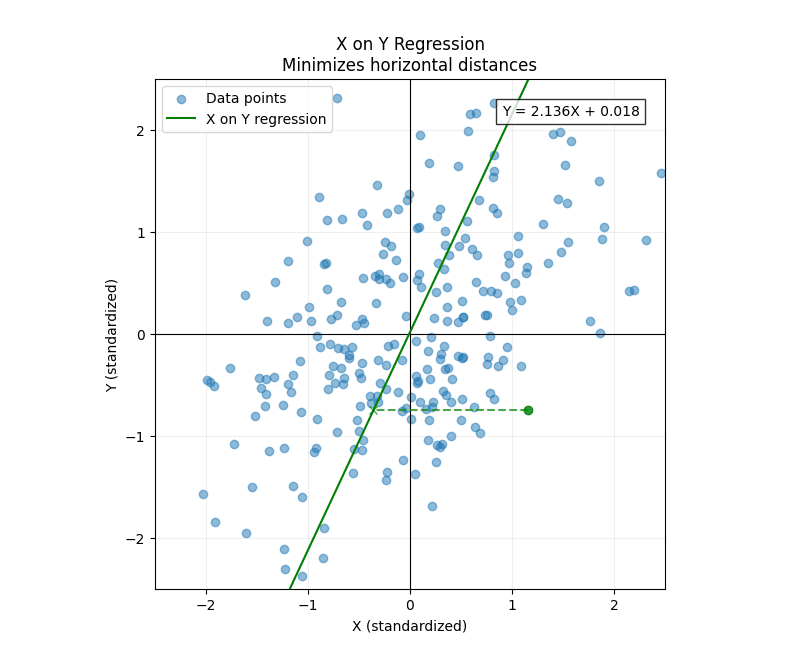
Now let's consider the converse case. When you regress $X$ onto $Y$, the roles of $X$ and $Y$ switch: our task becomes: "Given a value of $Y$, what is our best guess at the value of $X$"? In our example, that corresponds to the question: "Given the height of the son, what is our best guess at the height of the father?"

The cost function is now:

$$J_X\left({\beta }_X\right)=|X-{\beta }_{X}Y{|}^2$$

In this case, the errors are measured horizontally.

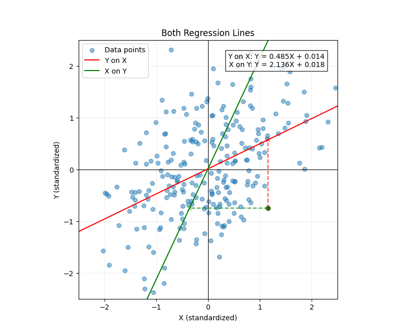
The two regression lines differ even though the data set is symmetric. Why?

Because each regression task measures errors in different directions. This explains not only why the two regression lines are different, but also the precise way they differ. Since least-squares is quadratic, it harshly punishes outliers. Therefore, the regression line for $Y$ onto $X$ will have less variation in the $Y$ direction because it needs to be conservative---that's why its slope is less than 1. Conversely, when we regress $X$ onto $Y$, the line will be compressed along the $X$ direction since it must be conservative along that axis. That's why its slope is greater than 1.

This becomes intuitive when we consider our example of father-son heights. If the father's height is 6 foot 3, our best guess for the son's height is 6 foot. This is given by our $Y$-on-$X$ regression line. And if the son's height is 6 foot 3, our best guess for the father's height is 6 foot. This is given by our $X$-on-$Y$ regression line.

We should expect to see regression to the mean regardless of whether we start with the father's height or the son's height. If the two regression lines were the same, then when the son's height is 6 foot, our best guess for the father's height would be 6 foot 3---which doesn't make sense.

I think misconceptions often arise because we have a (correct) intuition that a problem is "symmetric," but then hastily leap to the wrong symmetry. It's tempting to see the inherent symmetry in this problem (the marginal distributions for father and son are the same) and assume the regression lines should be mathematically the same.

However, the task itself breaks the symmetry by designating one variable as the input (which we know precisely) versus the output (which is uncertain and what we are trying to predict). There is still a symmetry present, though: the regression lines are symmetric about the line $y=x$.

Now we will consider principal component analysis. To borrow machine learning lingo: If linear regression is the grandfather of supervised learning, then principal component analysis is the grandfather of unsupervised learning. Instead of trying to predict one variable based on another, PCA aims to find the best model of the data's underlying structure.

If you squint a bit, you can see that our data sort of looks like an ellipse. A way to think about PCA geometrically is that the semi-major axis of this ellipse is the axis of the first principal component.

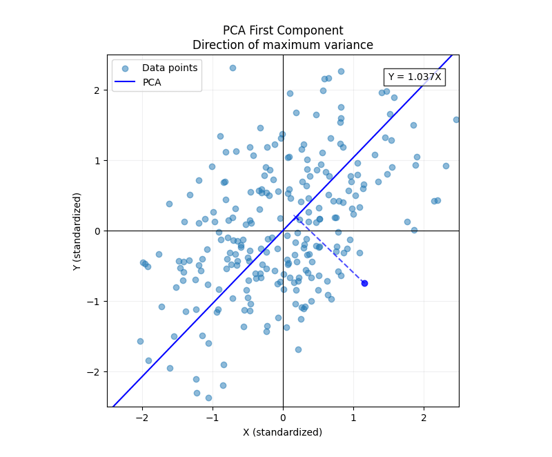
The PCA axis is the line $y=x$. This makes sense as, unlike with linear regression, the task doesn't break the symmetry between $x$ and $y$.

PCA is all about finding the direction that maximizes the variance of the data (as a proxy for explanatory power). It turns out that this is equivalent to finding the line that minimizes the sum of squared orthogonal projections. To show this equivalency, it's easiest to start with the orthogonal projection cost function.

This section will unfortunately require a bit more math than the previous sections. While linear regression lines are defined in terms of their minimizing cost functions, it will take more work to show that, for PCA, the orthogonal projection cost function is indeed the correct one.

Let $\overrightarrow{z}=(x,y)$ be a vector representing some data point, and let $\hat{v}$ be some unit vector in the $x-y$ plane. $\hat{v}$ represents a direction which we are projecting the data onto. It's a basic fact of linear algebra that we can decompose every data point into its component parallel to $\hat{v}$ and its component perpendicular to $\hat{v}$ (which we will call $\overrightarrow{w}$):

$$\overrightarrow{z}=(\overrightarrow{z}\cdot \hat{v})\hat{v}+\overrightarrow{w}$$

We want to minimize the squared magnitude of $\overrightarrow{w}$ when summed over every data point. But first, it helps to express $|\overrightarrow{w}{|}^2$ in a more convenient form. One can show that:

$$\begin{array}{cc}|\overrightarrow{w}{|}^2& =|\overrightarrow{z}-(\overrightarrow{z}\cdot \hat{v})\hat{v}{|}^2\\ & =(\overrightarrow{z}-(\overrightarrow{z}\cdot \hat{v}\left)\hat{v}\right)\cdot (\overrightarrow{z}-(\overrightarrow{z}\cdot \hat{v}\left)\hat{v}\right)\\ & =|\overrightarrow{z}{|}^2-(\overrightarrow{z}\cdot \hat{v}{)}^2\end{array}$$

If we define the cost function $J_{\text{PCA}}$ as the sum of these orthogonal projections, we have:

$$\begin{array}{cc}{J}_{\text{PCA}}\left(\hat{v}\right)& =\sum _{i=1}^N|w_i{|}^2\\ & =\sum _{i=1}^N|\overrightarrow{z_i}{|}^2-(\overrightarrow{z_i}\cdot \hat{v}{)}^2\\ & =-\sum _{i=1}^N(\overrightarrow{z_i}\cdot \hat{v}{)}^2+C\end{array}$$

In the last line, we used the fact that the sum of the squared lengths of the data points ${\overrightarrow{z}}_i$ is independent of the direction of projection. Minimizing the orthogonal projection cost function is equivalent to maximizing the sum of $(\overrightarrow{z_i}\cdot \hat{v}{)}^2$---which is precisely the variance of our data projected along the direction $\hat{v}$.

2 comments

Comments sorted by top scores.