Defining Optimization in a Deeper Way Part 2

post by J Bostock (Jemist) · 2022-07-11T20:29:30.225Z · LW · GW · 0 comments

Contents

  The Dumb Thermostat
  The Smart Thermostat
  Quantitative Data
  The Continuous Thermostat
  Where does this leave us?
None
No comments

We have successfully eliminated the concepts of null actions and nonexistence from our definition of optimization. We have also eliminated the concept of repeated action. We are halfway there, and now have to eliminate uncertainty and absolute time. Then we will have achieved the goal of being able to wrap a 3D hyperplane boundary around a 4D chunk of relativistic spacetime and ask ourselves "Is this an optimizer?" in a meaningful way.

I'm going to tackle uncertainty next.

TL;DR I have allowed for a mor

We've already defined, for a deterministic system, that a joint probability distribution $P_t^{AB}(s^A,s^B)$ has a numerical optimizing-ness, in terms of entropy. Now I want to extend that to a non-joint probability distribution of the form $P^A\left(s^A\right)P^B\left(s^B\right)$. We can do this by defining $P_{t-1}^A\left(s^A\right)$ and $P_{t-1}^B\left(s^B\right)$ for the previous timestep.

We can then define $P_t^{AB}(s^A,s^B)$ as by stepping forwards from $t-1$ to $t$ as before, according to the dynamics of the system.

A question we might want to ask is, for a given $P_{t-1}^A\left(s^A\right)$ and $P_{t-1}^B\left(s^B\right)$, how "optimizing" is the distribution $P_t^{AB}(s^A,s^B)$?

---

The Dumb Thermostat

Lets apply our new idea to the previous models, the two thermostats. Lets begin with uncorrelated, maximum entropy distributions.

For thermostat 1 we have the dynamic matrix:

	$hot$	$warm$	$cold$
$high$	$(hot,off)$	$(hot,low)$	$(warm,high)$
$low$	$(hot,off)$	$(warm,low)$	$(cold,high)$
$off$	$(warm,off)$	$(cold,low)$	$(cold,high)$

(In this matrix, the entry for a cell represents the state at $time=t+1$ given the coordinates of that cell represent the state at $time=t$)

With the $P_{t-1}^{RT}$ distribution:

	$hot$	$warm$	$cold$
$high$	$1/9$	$1/9$	$1/9$
$low$	$1/9$	$1/9$	$1/9$
$off$	$1/9$	$1/9$	$1/9$

As an aside this has 3.2 bits of entropy.

Leading to the $P_t^{RT}$

 distribution:

	$hot$	$warm$	$cold$
$high$	$0$	$1/9$	$2/9$
$low$	$1/9$	$1/9$	$1/9$
$off$	$2/9$	$1/9$	$0$

This gives us the "standard" $P_{t+1}^{RT}$ distribution of:

	$hot$	$warm$	$cold$
$high$	$0$	$2/9$	$1/9$
$low$	$1/9$	$1/9$	$1/9$
$off$	$1/9$	$2/9$	$0$

And the "decorrelated" $P_{t+1}^{\prime RT}$ distribution is actually just the same as $P_t^{RT}$! When we decorrelate the probabilities for $s^R$ and $s^T$ we just get back to the maximum entropy distribution and so $P_{t+1}^{\prime RT}=P_t^{RT}$

It's clear by inspection that the distributions $P_{t+1}^{RT}$ and $P_{t+1}^{\prime RT}$ have the same entropy, so the decorrelated maximum entropy $P_{t-1}^R{P}_{t-1}^T$ does not produce an "optimizing" distribution at $P_t^{RT}$.

If we actually consider the dynamics of this system, we can see that this makes sense! The temperature actually either stays at $(warm,low)$ or falls into the cycle:

$(hot,low)\to (hot,off)\to (warm,off)\to (cold,low)\to (cold,high)\to (warm,high)\to (hot,low)$

So there's no compression of futures into a smaller number of trajectories.

---

The Smart Thermostat

What about our "smarter" thermostat? This one has the dynamic matrix:

	$hot$	$warm$	$cold$
$high$	$(hot,off)$	$(hot,low)$	$(warm,low)$
$low$	$(hot,off)$	$(warm,low)$	$(cold,high)$
$off$	$(warm,low)$	$(cold,low)$	$(cold,high)$

Well now our $P_t^{RT}$ distribution looks like this:

	$hot$	$warm$	$cold$
$high$	$0$	$0$	$2/9$
$low$	$1/9$	$1/3$	$1/9$
$off$	$2/9$	$0$	$0$

Giving "standard" a $P_{t+1}^{RT}$ of this:

	$hot$	$warm$	$cold$
$high$	$0$	$0$	$1/9$
$low$	$0$	$7/9$	$0$
$off$	$1/9$	$0$	$0$

And a "decorrelated" $P_t^{\prime RT}$ of:

	$hot$	$warm$	$cold$
$high$	$2/27$	$2/27$	$2/27$
$low$	$5/27$	$5/27$	$5/27$
$off$	$2/27$	$2/27$	$2/27$

Giving the decorrelated $P_{t+1}^{\prime RT}$:

	$hot$	$warm$	$cold$
$high$	$0$	$0$	$7/27$
$low$	$2/27$	$1/3$	$2/27$
$off$	$7/27$	$0$	$0$

Now in this case, these two do have different entropies. $P_{t+1}^{RT}$ has an entropy of 1.0 bits, and $P_{t+1}^{\prime RT}$ has an entropy of 2.1 bits. This gives us a difference of 1.1 bits of entropy. This is the Optimizing-ness we defined in the last post, but I think it's actually somewhat incomplete.

Let's also consider the initial difference between $P_t^{RT}$ and $P_t^{\prime RT}$. Decorrelating $P_t^{RT}$ takes it from 2.2 to 3.0 bits of entropy. So the entropy difference started off at 0.8 bits. Therefore the difference of the difference in entropy is 0.3 bits.

The value of associated with $P_{t-1}^{RT}$ is equal to $\left(S\right[P_{t+1}^{\prime RT}]-S[P_{t+1}^{RT}\left]\right)-\left(S\right[P_t^{\prime RT}]-S[P_t^{RT}\left]\right)$. which can also be expressed as $S\left[P_{t+1}^{\prime RT}\right]+S\left[P_t^{RT}\right]-S\left[P_{t+1}^{RT}\right]-S\left[P_t^{\prime RT}\right]$. We might call this quantity the adjusted optimizing-ness.

---

Quantitative Data

The motivation for this was that a maximum entropy distribution is "natural" in some sense. This moves us towards not needing uncertainty. If we have a given state of a system, we might be able to "naturally" define a probability distribution around that state. Then we can measure the optimizing-ness of the next step's distribution.

What happens with a different $P_{t-1}^{RT}$ condition? What if we have a distribution like this:

	$hot$	$warm$	$cold$
$high$	${ϵ}^2/4$	$ϵ(1-ϵ)/2$	${ϵ}^2/4$
$low$	$ϵ(1-ϵ)/2$	$(1-ϵ{)}^2$	$ϵ(1-ϵ)/2$
$off$	${ϵ}^2/4$	$ϵ(1-ϵ)/2$	${ϵ}^2/4$

For some small epsilon in the second situation.

Now $P_t^{RT}$ is like this:

	$hot$	$warm$	$cold$
$high$	$0$	$0$	$ϵ(1-ϵ)/2+{ϵ}^2/4$
$low$	$ϵ(1-ϵ)/2$	$(1-ϵ{)}^2+{ϵ}^2/2$	$ϵ(1-ϵ)/2$
$off$	$ϵ(1-ϵ)/2+{ϵ}^2/4$	$0$	$0$

So $P_{t+1}^{RT}$ is:

	$hot$	$warm$	$cold$
$high$	$0$	$0$	$ϵ(1-ϵ)/2$
$low$	$0$	$1-ϵ(1-ϵ)$	$0$
$off$	$ϵ(1-ϵ)/2$	$0$	$0$

While it is theoretically possible to decorrelate everything, calculate the next set of things, and keep going, it's a huge mess. Using values for epsilon between 0.1 and ${10}^{-10}$ we can make the following plot between the entropy of $P_{t-1}^{RT}$ and our previously defined adjusted optimizing-ness.

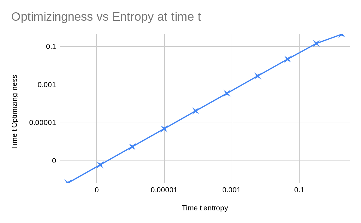
It looks linear in the log/log particularly in the region where $ϵ$ is very small. By fitting to the leftmost five points we get a simple linear relation: The adjusted optimizing-ness approaches half of the entropy of $P_{t-1}^{RT}$.

This is kind of weird. This might not be an optimal system to study, so let's look at another toy example. A more realistic model of a thermostat:

---

The Continuous Thermostat

The temperature of the room is considered as $S^R\in R$. The activity of the thermostat is considered as $T\in R$. Each timestep, we have the following updates:

$S_{t+1}^T=S_t^R$

$S_{t+1}^R=S_t^R-k{S}_t^T$

Consider the following distributions:

$P_{t-1}^R\left(s^R\right)\sim U(10-ϵ/2,10+ϵ/2)$

$P_{t-1}^T\left(s^T\right)\sim U(10-ϵ/2,10+ϵ/2)$

Where $U(a,b)$ refers to a uniform distribution between $a$ and $b$. $P_{t-1}^{RT}$ can be thought of as a square of side length $ϵ$ centered on the point $(10,10)$. $P_t^{RT}$ turns out to be a rhombus. The corners transform like this:

Time = $t-1$	Time = $t$
$(10+ϵ,10+ϵ)$	$\left(10\right(1-k)+ϵ(1-k),10+ϵ)$
$(10+ϵ,10-ϵ)$	$\left(10\right(1-k)+ϵk,10+ϵ)$
$(10-ϵ,10+ϵ)$	$\left(10\right(1-k)-ϵk,10-ϵ)$
$(10-ϵ,10-ϵ)$	$\left(10\right(1-k)-ϵ(1-k),1-ϵ)$

For $ϵ=0.1,k=0.3$ the whole sequence looks like the following:

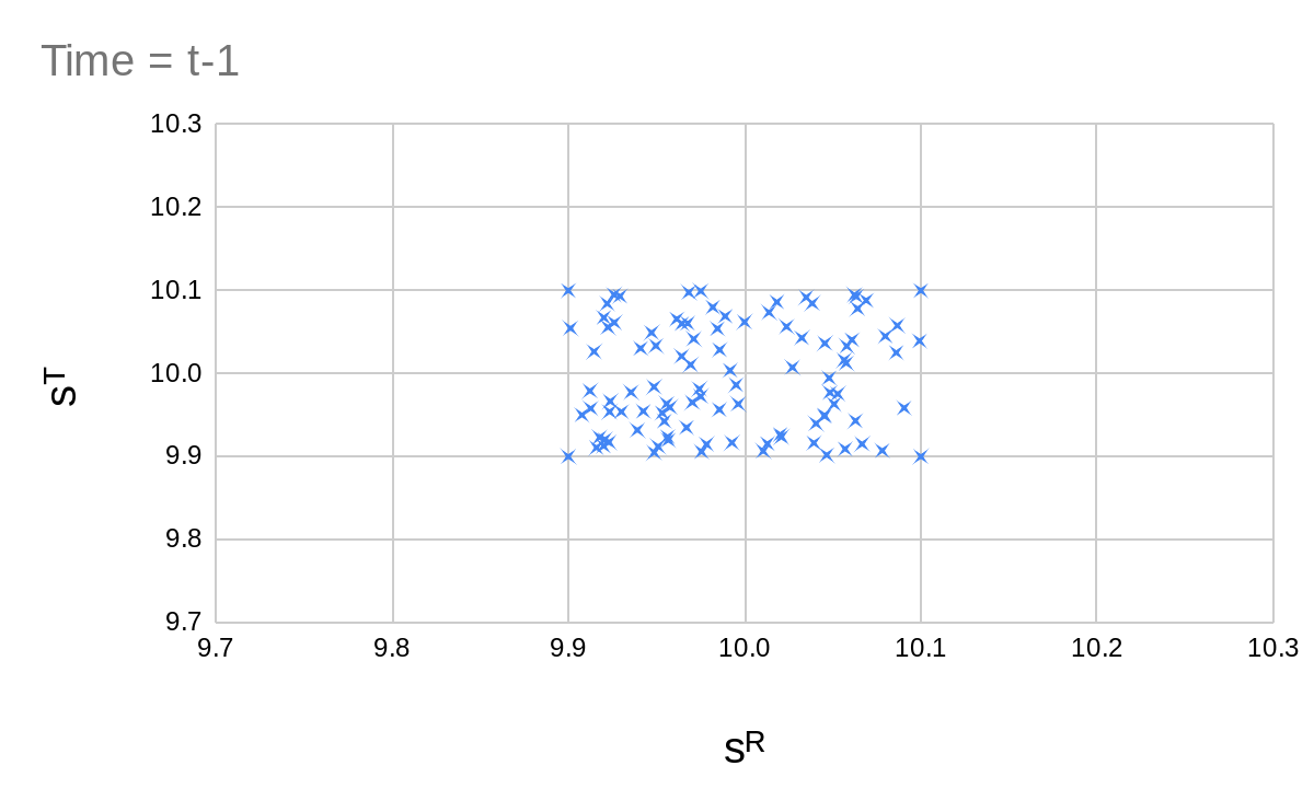
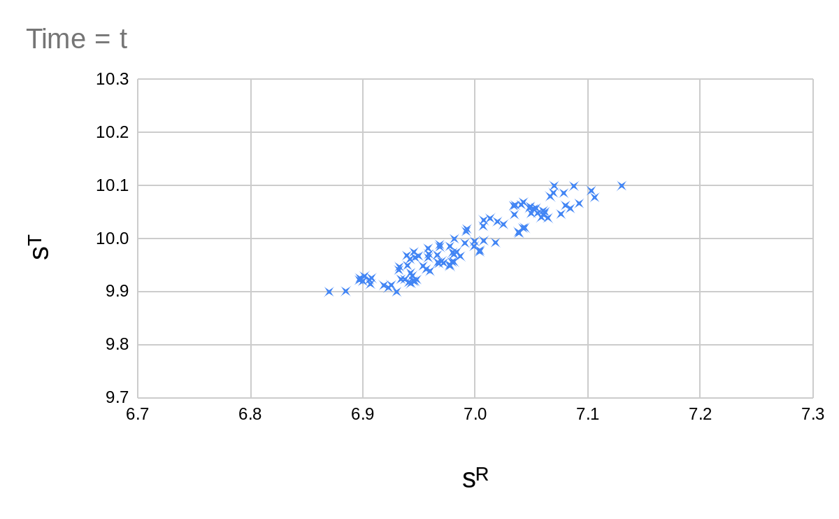
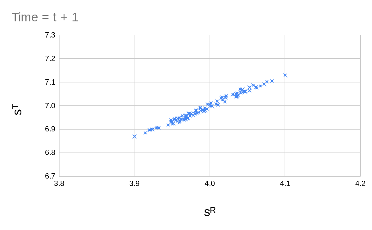
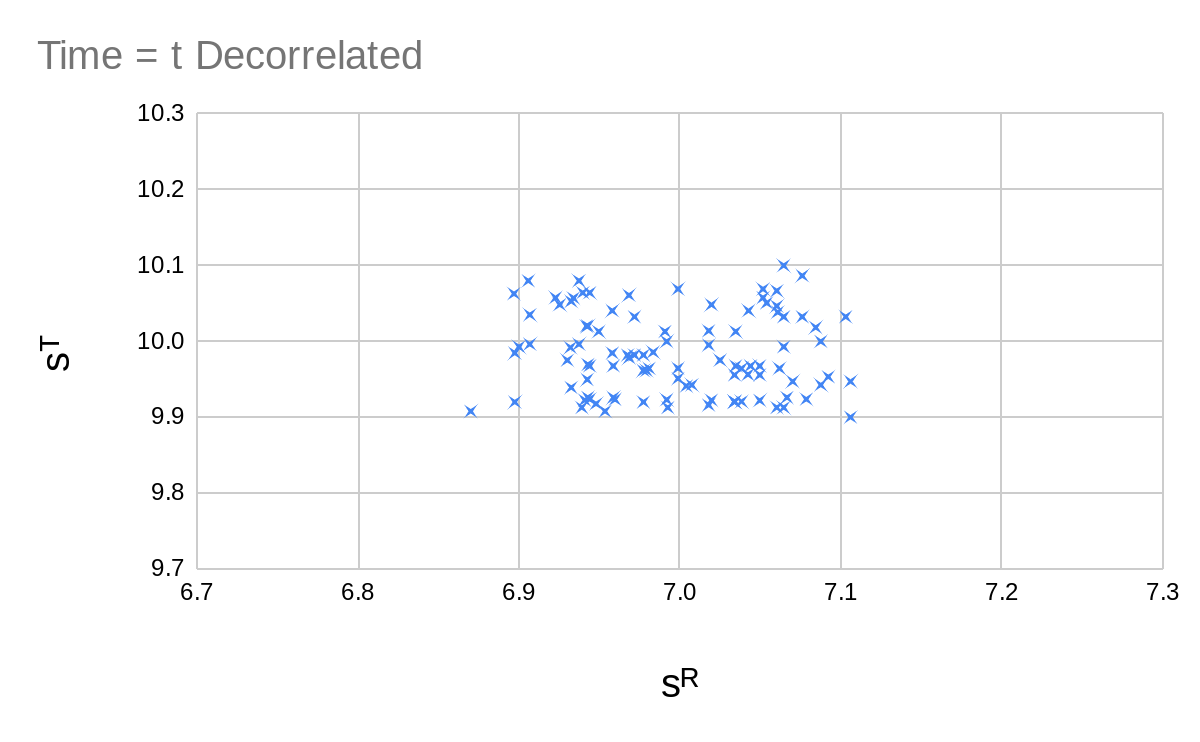
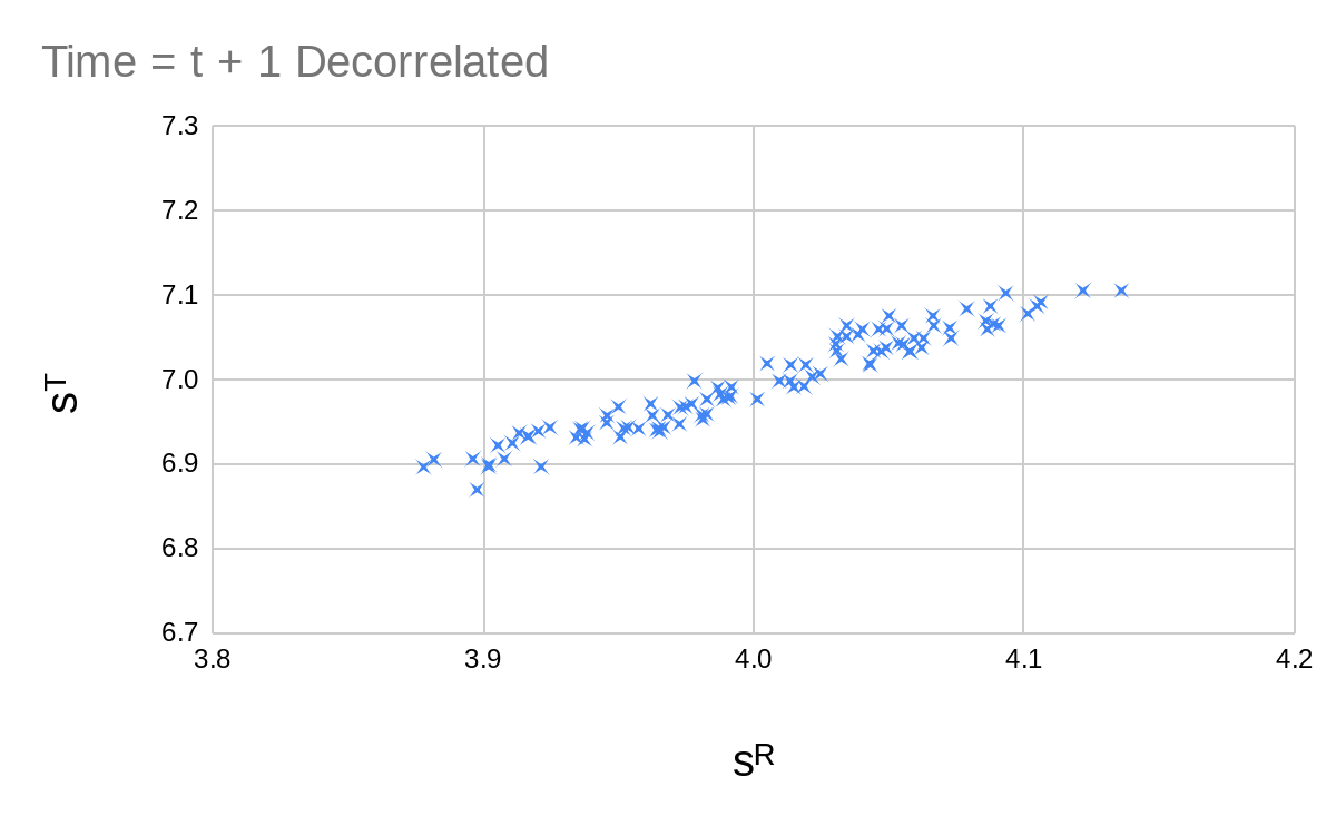
So we clearly have some sort of optimization going on here. Estimating or calculating the entropy of these distributions is not easy. And when we use the entropy of a continuous distribution, we get results which depend on the choice of coordinates (or alternatively the choice of some weighting function). Entropies of continuous distributions may also be negative, which is quite annoying.

Perhaps calculating the variance will leave us better off? Sadly not. I tried it for gaussians of decreasing variance and didn't get much. The equivalent to our adjusted optimizing-ness which we might define as $log\left(V\right[P_{t+1}^{\prime AB}\left]\right)+log\left(V\right[P_t^{AB}\left]\right)-log\left(V\right[P_t^{\prime AB}\left]\right)-log\left(V\right[P_{t+1}^{AB}\left]\right)$ is always zero for this system. The non-adjusted version $log\left(V\right[P_{t+1}^{\prime AB}\left]\right)-log\left(V\right[P_{t+1}^{AB}\left]\right)$ fluctuates a lot.

---

Where does this leave us?

We can define whether something is an optimizer based on a probability distribution which need not be joint over $A$ and $B$. This means we can define whether something is an optimizer for an arbitrarily narrow probability distribution, meaning we can take the limit as the probability distribution approaches a delta. We found an interesting relation between quantities in our simplified system but failed to extend it to a continuous system.

0 comments

Comments sorted by top scores.