Ophiology (or, how the Mamba architecture works)

post by Danielle Ensign (phylliida-dev), SrGonao (srgonao), Adrià Garriga-alonso (rhaps0dy) · 2024-04-09T19:31:09.975Z · LW · GW · 8 comments

Contents

  A new challenger arrives!
    Promising Scaling
    Efficient Inference
  What are State-space models?
  Solving the ODE
    Euler method
    Zero-Order Hold (ZOH)
    Discretization rule used in Mamba
  Specific Quirks to Mamba
    The structured SSM
      The case of a 1-Dimensional input
      The Mamba implementation
    Selection mechanism
    WΔ is low rank
    RMSNorm
  Full Architecture
    Dimensions
    Notes on reading these graphs
    Overview
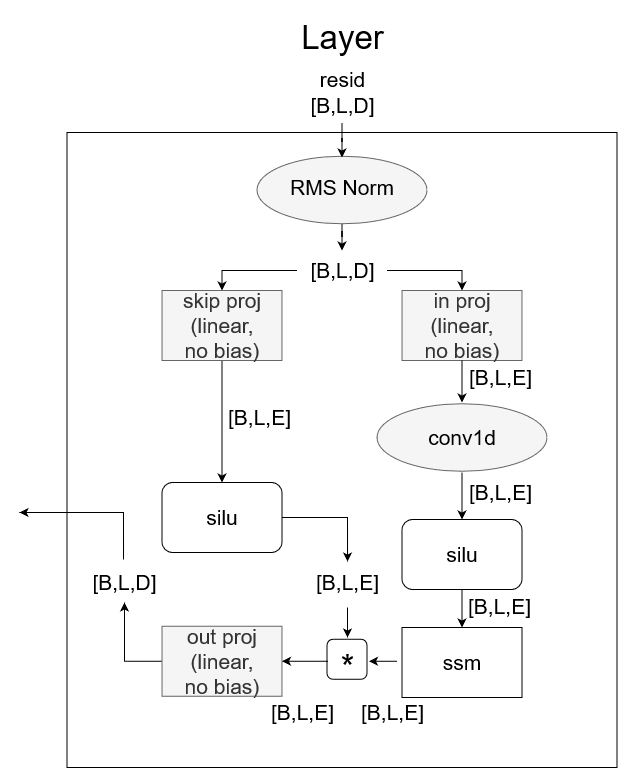
    Layer contents
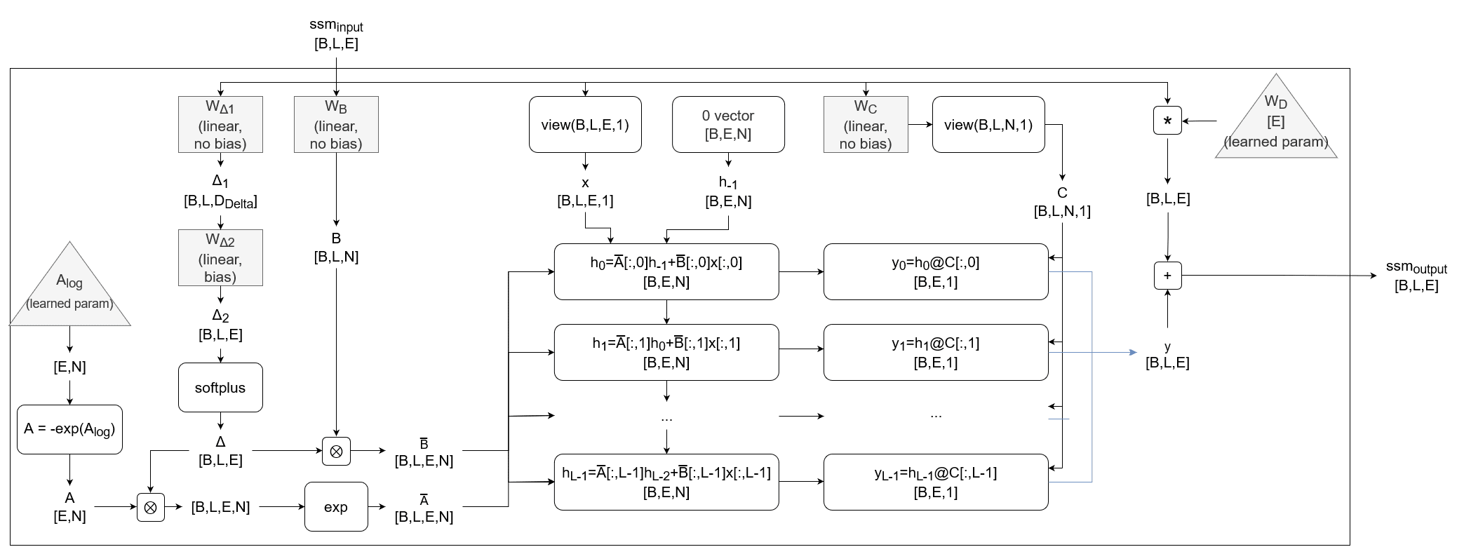
    SSM
  Further reading
  Appendix
    Conv1D Explanation
    Worked Conv Example
    Conv1D in code
None
8 comments

The following post was made as part of Danielle's MATS work on doing circuit-based mech interp on Mamba, mentored by Adrià Garriga-Alonso. It's the first in a sequence of posts about finding an IOI circuit in Mamba/applying ACDC to Mamba.

This introductory post was also made in collaboration with Gonçalo Paulo.

A new challenger arrives!

Why Mamba?

Promising Scaling

Mamba ^[1] is a type of recurrent neural network based on state-space models, and is being proposed as an alternative architecture to transformers. It is the result of years of capability research ^{[2] [3] [4]} and likely not the final iteration of architectures based on state-space models.

In its current form, Mamba has been scaled up to 2.8B parameters on The Pile and on Slimpj, having similar scaling laws when compared to Llama-like architectures.

            Scaling curves from Mamba paper: Mamba scaling compared to Llama (Transformer++), previous state space models (S3++), convolutions (Hyena), and a transformer inspired RNN (RWKV)

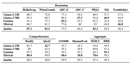
More recently, ai21labs ^[5] trained a 52B parameter MOE Mamba-Transformer hybrid called Jamba. At inference, this model has 12B active parameters and has benchmark scores comparable to Llama-2 70B and Mixtral.

            Jamba benchmark scores, from Jamba paper ^[5:1]

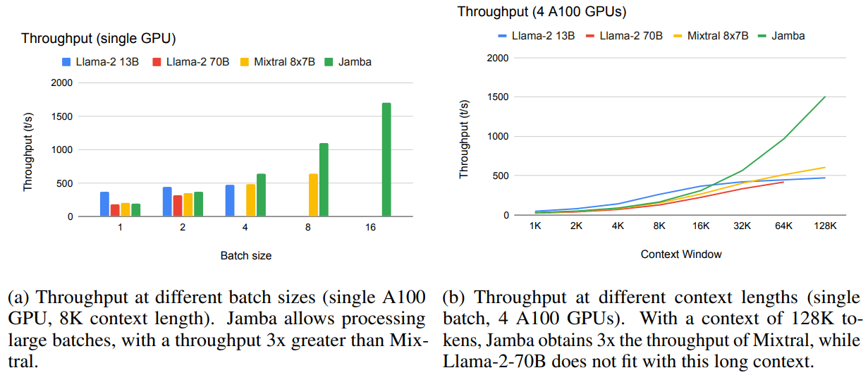
Efficient Inference

One advantage of RNNs, and in particular of Mamba, is that the memory required to store the context length is constant, as you only need to store the past state of the SSM and of the convolution layers, while it grows linearly for transformers. The same happens with the generation time, where predicting each token scales as $O\left(1\right)$ instead of $O\left(\text{context length}\right)$.

            Jamba throughput (tokens/second), from Jamba paper^[5:2]

What are State-space models?

The inspiration for Mamba (and similar models) is an established technique used in control theory called state space models (SSM). SSMs are normally used to represent linear systems that have p inputs, q outputs and n state variables. To keep the notation concise, we will consider the input as E-dimensional vector $x\left(t\right)\in R^E$, an E-dimensional output $y\left(t\right)\in R^E$ and a N-dimensional latent space $h\in R^N$. In the following, we will note the dimensions of new variables using the notation [X,Y]. In particular, in Mamba 2.8b, E=5120 and N=16.

Specifically, we have the following:

$$\stackrel{\left[N\right]}{\dot{h}\left(t\right)}=\stackrel{[N,N]}{A}\stackrel{\left[N\right]}{h\left(t\right)}+\stackrel{[N,E]}{B}\stackrel{\left[E\right]}{x\left(t\right)}$$ $$\stackrel{\left[E\right]}{y\left(t\right)}=\stackrel{[E,N]}{C}\stackrel{\left[N\right]}{h\left(t\right)}+\stackrel{[E,E]}{D}\stackrel{\left[E\right]}{x}\left(t\right)$$

This is an ordinary differential equation (ODE), where $\dot{h}\left(t\right)$ is the derivative of $h\left(t\right)$ with respect to time, t. This ODE can be solved in various ways, which will be described below.

In state space models, $A$ is called the state matrix, $B$ is called the input matrix, $C$ is called the output matrix, and $D$ is called the feedthrough matrix.

Solving the ODE

We can write the ODE from above as a recurrence, using discrete timesteps:

$$\stackrel{\left[N\right]}{h_t}=\stackrel{[N,N]}{\overline{A}}\stackrel{\left[N\right]}{h_{t-1}}+\stackrel{[N,E]}{\overline{B}}\stackrel{\left[E\right]}{x_t}$$ $$\stackrel{\left[E\right]}{y_t}=\stackrel{[E,N]}{C}\stackrel{\left[N\right]}{h_t}+\stackrel{[E,E]}{D}{\stackrel{\left[E\right]}{x}}_t$$

where $\overline{A}$ and $\overline{B}$ are our discretization matrices. Different ways of integrating the original ODE will give different $\overline{A}$ and $\overline{B}$, but will still preserve this overall form.

In the above, $t$ corresponds to discrete time. In language modeling, $t$ refers to the token position.

Euler method

The simplest way to numerically integrate an ODE is by using the Euler method, which consists in approximating the derivative by considering the ratio between a small variation in h and a small variation in time, $\dot{h}=\frac{dh}{dt}\approx \frac{\Delta h}{\Delta t}$. This allows us to write:

$$\frac{h_{t+1}-h_t}{\Delta t}=A{h}_t+B{x}_t$$ $$h_{t+1}=\Delta t(A{h}_t+B{x}_t)+h_t$$

Where the index t, of $h_t$, represents the discretized time. This is the similar to when considering a character's position and velocity in a video game, for instance. If a character has a velocity $v$ and a position $x_0$, to find the position after $\Delta t$ time we can do $x_1=\Delta tv+x_0$. In general:

$$x_t=\Delta t{v}_t+x_{t-1}$$

Turning back to the above example, we can rewrite

$$h_{t+1}=\Delta t(A{h}_t+B{x}_t)+h_t$$

as

$$h_t=(\Delta A+I)h_{t-1}+\Delta B{x}_t$$

which means that, for the Euler Method, $\overline{A}=(\Delta A+I)$ and $\overline{B}=\Delta B$.

Here, $\Delta$ is an abbreviation of $\Delta t$, the discretization size in time.

Zero-Order Hold (ZOH)

Another way to integrate the ODE is to consider that the input $x\left(t\right)$ remains fixed during a time interval $\Delta$, and to integrate the differential equation from time $t$ to $t+\Delta$. This gives us an expression for $x(t+\Delta )$:

$$x(t+\Delta )=e^{\Delta A}x\left(t\right)+u(t+1){\int }_t^{t+\Delta }{e}^{(t+\Delta -\tau )A}Bd\tau$$

With some algebra we finally get:

$$\overline{A}=\exp \left(\Delta A\right)\overline{B}=\left(\Delta A{)}^{-1}\right(\exp \left(\Delta A\right)-I)\Delta B$$

Discretization rule used in Mamba

Mamba uses a mix of Zero-Order Hold and the Euler Method:

$$\overline{A}=\exp \left(\Delta A\right)\overline{B}=\Delta B$$

Why is this justified? Consider the ZOH $\overline{B}$:

$$\overline{B}=\left(\Delta A{)}^{-1}\right(\exp \left(\Delta A\right)-I)\Delta B$$

In Mamba, $A$ is diagonal, as we will see later, so we can write

$$(\left(\Delta A{)}^{-1}\right(\exp \left(\Delta A\right)-I){)}_{i,i}=\frac{\exp \left(\Delta A_{i,i}\right)-1}{\Delta A_{i,i}}$$

If we consider that $\Delta A_{i,i}$ is small and we expand the exponential to just first order ^[6], this expression reduces to 1 which means that:

$$\overline{B}=\left(\Delta A{)}^{-1}\right(\exp \left(\Delta A\right)-I)\Delta B\approx \Delta B$$

for small enough $\Delta A_{i,i}$. Using the same approximation for $\overline{A}$ recovers the Euler method:

$$\overline{A}=\exp \left(\Delta A\right)\approx I+\Delta A$$

In the original work, the authors argued that while ZOH was necessary for the modeling of $\overline{A}$, using the Euler Method for $\overline{B}$ gave reasonable results, without having to compute $(\Delta A{)}^{-1}$.

Specific Quirks to Mamba

The structured SSM

Mamba takes an interesting approach to the SSM equation. As previously mentioned, each timestep in Mamba represents a token position, and each token is represented (by the time it arrives to the SSM) by a E dimensional vector. The authors chose to represent the SSM as:

$$\stackrel{[E,N]}{h_t}=\stackrel{[E,N]}{\overline{A}}\stackrel{[E,N]}{h_{t-1}}+\stackrel{[E,N]}{\overline{B}}\stackrel{\left[E\right]}{x_t}$$

$$\stackrel{\left[E\right]}{y_t}=\stackrel{\left[N\right]}{C}\stackrel{[E,N]}{h_t}+\stackrel{\left[E\right]}{D}\stackrel{\left[E\right]}{x_t}$$

The case of a 1-Dimensional input

When trying to understand Mamba, I find it's easiest to start with each $x_t$ being a single value first, and then working up from there. The standard SSM equation is, then:

$$\stackrel{\left[N\right]}{h_t}=\stackrel{[N,N]}{\overline{A}}\stackrel{\left[N\right]}{h_{t-1}}+\stackrel{[N,1]}{\overline{B}}\stackrel{\left[1\right]}{x_t}$$ $$\stackrel{\left[1\right]}{y_t}=\stackrel{[1,N]}{C}\stackrel{\left[N\right]}{h_t}+\stackrel{[1,1]}{D}{\stackrel{\left[1\right]}{x}}_t$$

The authors of the original Mamba paper were working on top of previous results on Structured SSMs. Because of this, in this work, A is a diagonal matrix. This means that A can be represented as a set of N numbers instead of a $NxN$ matrix. That gives us:

$$\stackrel{\left[N\right]}{h_t}=\stackrel{\left[N\right]}{\overline{A}}\stackrel{\left[N\right]}{h_{t-1}}+\stackrel{[N,1]}{\stackrel{\left[1\right]}{x_t}}$$ $$\stackrel{\left[1\right]}{y_t}=\stackrel{[1,N]}{C}\stackrel{\left[N\right]}{h_t}+\stackrel{[1,1]}{D}{\stackrel{\left[1\right]}{x}}_t$$

Where $\stackrel{\left[N\right]}{\overline{A}}\stackrel{\left[N\right]}{h_{t-1}}$ is an element-wise product. In this example we are mapping a $1$-dimensional input to a $n$-dimensional hidden state, then mapping the $n$-dimensional hidden state back to a $1$ dimensional output.

The Mamba implementation

In practice, $x_t$ and $y_t$ are not one dimensional, but $E$-dimensional vectors. Mamba simply maps each of these elements separately to a $N$ dimensional hidden space. So we can write a set of E equations:

$$\stackrel{\left[N\right]}{h_{t,e}}=\stackrel{\left[N\right]}{\overline{A}}\stackrel{\left[N\right]}{h_{t-1,e}}+\stackrel{[N,1]}{\overline{B}}\stackrel{\left[1\right]}{x_{t,e}}$$ $$\stackrel{\left[1\right]}{y_{t,e}}=\stackrel{[1,N]}{C}\stackrel{\left[N\right]}{h_{t,e}}+\stackrel{[1,1]}{D}{\stackrel{\left[1\right]}{x}}_{t,e}$$

Where $e$ ranges from $[1,E]$. This means that each dimension of input to the SSM block is modeled by its own, independent, SSM. We will see that, due to the selection mechanism (see below) $\Delta ,\overline{A},\overline{B},C$ are a function of all the dimensions of the input, not just the dimension e.

One thing to note: In practice, $A$ has a separate value for each $e$, and is encoded as an $[E,N]$ matrix. We can denote $\overline{A_e}=\Delta A_e$ as the $N$-sized entry for stream $e$, giving us,

$$\stackrel{\left[N\right]}{h_{t,e}}=\stackrel{\left[N\right]}{\overline{A_e}}\stackrel{\left[N\right]}{h_{t-1,e}}+\stackrel{[N,1]}{\overline{B}}\stackrel{\left[1\right]}{x_{t,e}}$$

Selection mechanism

Mamba deviates from the simplest SSM approaches, and from the previous work of the authors, by making matrices B and C dependent on the input, x(t). Not only that, but the time discretization $\Delta$ is also input dependent. This replaces the equations shown above, with one which takes the form:

$$\stackrel{\left[N\right]}{h_{t,e}}=\stackrel{\left[N\right]}{\overline{A_{t,e}}}\stackrel{\left[N\right]}{h_{t-1,e}}+\stackrel{[N,1]}{\overline{B_{t,e}}}\stackrel{\left[1\right]}{x_{t,e}}$$ $$\stackrel{\left[1\right]}{y_{t,e}}=\stackrel{[1,N]}{C_t}\stackrel{\left[N\right]}{h_{t,e}}+\stackrel{[1,1]}{D}{\stackrel{\left[1\right]}{x}}_{t,e}$$

Where the new matrices are given by:

$$\stackrel{\left[N\right]}{\overline{A_{t,e}}}=\exp \left(\stackrel{\left[1\right]}{{\Delta }_{t,e}}\stackrel{\left[N\right]}{A_e}\right)$$

$$\stackrel{\left[N\right]}{\overline{B_{t,e}}}=\stackrel{\left[1\right]}{{\Delta }_{t,e}}\stackrel{\left[N\right]}{B_t},\text{with}\stackrel{\left[N\right]}{B_t}=\stackrel{[N,E]}{W_B}\stackrel{\left[E\right]}{x_t}$$

$$\stackrel{\left[N\right]}{C_t}=\stackrel{[N,E]}{W_C}\stackrel{\left[E\right]}{x_t}$$

$$\stackrel{\left[1\right]}{{\Delta }_{t,e}}=\text{softplus}(\stackrel{\left[E\right]}{x_t}\cdot \stackrel{\left[E\right]}{W_e^{\Delta }}+\stackrel{\left[1\right]}{B_e^{\Delta }})$$

with $\stackrel{[E,E]}{W^{\Delta }},\stackrel{\left[E\right]}{B^{\Delta }},\stackrel{[N,E]}{W_B},\stackrel{[N,E]}{W_C}$ being learned parameters, and $\text{softplus}\left(x\right)=\log (1+e^x)$

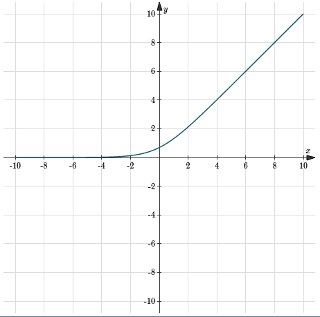
                                                softplus

One final thing to note: A is not a trainable parameter, and what is actually trained is ${\stackrel{[E,N]}{A}}_{\text{log}}$. $A$ is then computed as $A=-exp\left(A_{\text{log}}\right)$ (using element-wise exp). This ensures $A$ is a strictly negative number. Because $\Delta$ is always postitive, this ensures that the first term of SSM can be seen as how much of the previous state is kept at a given token position, while the second term is related to how much it is written to the state.

In turn, this implies that $\exp \left(\Delta A\right)$ is between 0 and 1. This is important for stable training: it ensures that the elements of $h\left(t\right)$ do not grow exponentially with token position $t$, and the gradients do not explode. It is long known ^[7] that the explosion and vanishing of gradients are obstacles to training RNNs, and successful architectures (LSTM, GRU) minimize these.

$W_{\Delta }$ is low rank

In Mamba, they don't encode $\stackrel{[E,E]}{W_{\Delta }}$ as an $[E,E]$ matrix. Instead, it is encoded as two smaller matrices:

$$\stackrel{[E,E]}{W_{\Delta }}=\stackrel{[E,D_{\Delta }]}{W_{{\Delta }_1}}\stackrel{[D_{\Delta },E]}{W_{{\Delta }_2}}$$

Where, for example, $E=2048$, $D_{\Delta }=64$

This makes this term

$$\stackrel{\left[1\right]}{{\Delta }_{t,e}}=\text{softplus}(\stackrel{\left[E\right]}{x_t}\cdot \stackrel{\left[E\right]}{W_{\Delta }[:,e]}+\stackrel{\left[1\right]}{B_{\Delta }\left[e\right]})$$

Be instead

$$\stackrel{\left[1\right]}{{\Delta }_{t,e}}=\text{softplus}(\stackrel{\left[1\right]}{\stackrel{}{\stackrel{\left[E\right]}{x_t}\cdot \stackrel{\left[E\right]}{\stackrel{}{(\stackrel{[E,D_{\Delta }]}{W_{{\Delta }_1}}\stackrel{\left[D_{\Delta }\right]}{W_{{\Delta }_2}[:,e]})}}}}+\stackrel{\left[1\right]}{B_{\Delta }\left[e\right]})$$

RMSNorm

This normalization is not unique to Mamba. It's defined as

$$RMSNorm\left(\stackrel{[B,L,D]}{x}\right)=\frac{x}{\sqrt{\text{mean}(x^2,\text{dim=-1})}}\text{weight}$$

If $\text{mean}$ was instead $\text{sum}$, this first term would be normalizing $x$ along the $D$ dimension. Because it's $\text{mean}$ there's an extra $D$ term, and we can rewrite this as:

$$RMSNorm\left(\stackrel{[B,L,D]}{x}\right)=\sqrt{D}\frac{x}{\sqrt{\text{sum}(x^2,\text{dim=-1})}}\text{weight}$$

The reason we want to do this is so that each element's value is on average 1, as opposed to the whole activation's vector. Since the introduction of the He initialization ^[8], deep learning weights have been initialized so the activation variance is 1 assuming the input variance is 1, thus keeping gradients stable throughout training.

Full Architecture

Now that we know how the SSM works, here is the full architecture.

Dimensions

(Example values from state-spaces/mamba-370m)

• $B$ is the batch size
• $L$ is the context length
• $D=d_{\text{model}}=1024$ is the dimension of the residual stream
• $E=d_{\text{inner}}=2048$ is the dimension of the embed size
• $N=d_{\text{state}}=16$ is the dimension of the state space
• $D_{\text{delta}}=d{t}_{\text{rank}}=64$ is the low rank size used when calculating delta, see section 4.4

Notes on reading these graphs

• Text not in circles/squares are variable names/size annotations
• Rounded, white rectangles are mathmatical operations
• Shaded triangles are learned params
• Shaded squares are learned params that are projections
• Shaded circles are conv or rms norm (other operations that have some learned params)

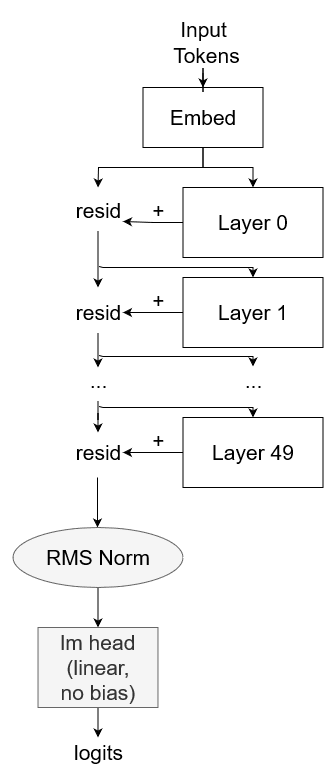
Overview

Mamba has:

• Embedding
• Residual stream that each layer adds to
• RMSNorm
• Project to logits

                 High level overview of Mamba

# [B,L,D]                 [B,L]
resid  = mamba.embedding(input_ids)
for layer in mamba.layers:
   # [B,L,D]     [B,L,D]
   resid += layer(resid)
# [B,L,D]              [B,L,D]
resid     = mamba.norm( resid )
# [B,L,V]           [D->V] [B,L,D]
logits    = mamba.lm_head( resid ) # no bias
return logits

Layer contents

Each layer does:

• Project input $\stackrel{[B,L,D]}{\text{resid}}$ to $\stackrel{[B,L,E]}{x}$
• Project input $\stackrel{[B,L,D]}{\text{resid}}$ to $\stackrel{[B,L,E]}{\text{skip}}$
• Conv over the $E$ dimension (see Appendix) ($x=\text{conv}\left(x\right)$)
• Apply non-linearity (silu) ($x=\text{silu}\left(x\right)$)
• $y=SSM\left(x\right)$
• Gating: $y=y\ast \text{silu}\left(\text{skip}\right)$
• Project $\stackrel{[B,L,E]}{y}$ to $\stackrel{[B,L,D]}{\text{output}}$

                                                              Mamba layer overview

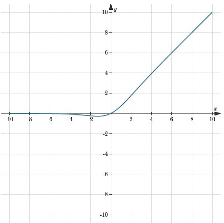
                                                  silu

def forward(layer, resid):
   ## Process inputs ##
   # [B,L,D]  [B,L,D]
   x         = resid
   # [B,L,D]             [B,L,D]
   x         = layer.norm(  x  )
   # [B,L,E]         [D->E]  [B,L,D]
   skip      = layer.skip_proj(  x  ) # no bias
   # [B,L,E]         [D->E] [B,L,D]
   x         = layer.in_proj(  x  ) # no bias
   
   ## Conv ##
   # [B,E,L]
   x         = rearrange(x, 'B L E -> B E L')
   # [B E L]                [B,E,L]  conv1d outputs [B,E,3+L], cut off last 3
   x         = layer.conv1d(   x   )[:, :, :L]
   # [B,L,E]
   x         = rearrange(x, 'B E L -> B L E')

   ## Non-linearity ##
   # silu(x) = x * sigmoid(x)
   # silu(x) = x * 1/(1+exp(-x))
   # [B,L,E]         [B,L,E]
   x         = F.silu(  x  ) 
   
   ## SSM ##
   # [B,L,E]               [B,L,E]
   y         = ssm( layer,    x    )

   ## Gating ##
   # [B,L,E]  [B,L,E]          [B,L,E]
   y         =   y      * F.silu(  skip  )

   ## Project out ##
   # [B,L,D]          [E->D]  [B,L,E]
   y         = layer.out_proj(   y   ) # no bias
   return y

SSM

From above:

$$\stackrel{\left[1\right]}{{\Delta }_{t,e}}=\text{softplus}(\stackrel{\left[E\right]}{x_t}\cdot (\stackrel{[E,D_{\Delta }]}{W_{{\Delta }_1}}\stackrel{[D_{\Delta },1]}{W_{{\Delta }_2}[:,e].\text{view}(D_{\Delta },1)}).\text{view}(E)+\stackrel{\left[1\right]}{B_{\Delta }\left[e\right]})$$

$$\stackrel{[E,N]}{A}=-\exp \left(\stackrel{[E,N]}{A_{log}}\right)$$

$$\stackrel{\left[N\right]}{\overline{A_{t,e}}}=\exp \left(\stackrel{\left[1\right]}{{\Delta }_{t,e}}\stackrel{\left[N\right]}{A_e}\right)$$

$$\stackrel{\left[N\right]}{B_t}=\stackrel{[N,E]}{W_B}\stackrel{\left[E\right]}{x_t}$$

$$\stackrel{\left[N\right]}{\overline{B_{t,e}}}=\stackrel{\left[1\right]}{{\Delta }_{t,e}}\stackrel{\left[N\right]}{B_t}$$

$$\stackrel{\left[N\right]}{C_t}=\stackrel{[N,E]}{W_C}\stackrel{\left[E\right]}{x_t}$$

$$\stackrel{\left[N\right]}{h_{t,e}}=\stackrel{\left[N\right]}{\overline{A_{t,e}}}\stackrel{\left[N\right]}{h_{t-1,e}}+\stackrel{[N,1]}{\overline{B_{t,e}}}\stackrel{\left[1\right]}{x_{t,e}}$$ $$\stackrel{\left[1\right]}{y_{t,e}}=\stackrel{[1,N]}{C_t}\stackrel{\left[N\right]}{h_{t,e}}+\stackrel{[1,1]}{D}{\stackrel{\left[1\right]}{x}}_{t,e}$$

where $\stackrel{[E,E]}{W_{\Delta }},\stackrel{\left[E\right]}{B_{\Delta }},\stackrel{[N,E]}{A_{log}},\stackrel{[N,E]}{W_B},\stackrel{[N,E]}{W_C}$ are learned parameters, and $\text{softplus}\left(x\right)=\log (1+e^x)$

def ssm(layer, x):
       
   # stored as A_log
   layer.A = -torch.exp(layer.A_log)
   
   ys = []
   # every (e) has a 1-D ssm
   for e in range(E):
       ys_e = []
       
       # latent state, init to zeros
       h_e = torch.zeros(Batch,N)
       for l in range(L):
           #### First, discretization: A and B -> Abar and Bbar ####
           ## Compute Delta ##
           # [E,1]  [E,D_Delta]                                [D_delta,1]
           inner_term = layer.W_delta_1.weight.T@layer.W_delta_2.weight.T[:,e].view(D_Delta,1)
           # [1]                 [E]             [E]                   [1]
           delta = F.softplus(x[:,e].dot(inner_term.view(E)) + layer.W_delta_2.bias[e])
           
           ## Discretize A ##
           # [B,N]             ( [B,1]  *   [N]    ) 
           A_bar     = torch.exp(delta * layer.A[e])
           
           ## Discretize B ##
           # [B,N]         [E->N] [B,E]
           B         = layer.W_B(x[b,l]) # no bias
           # [B,N]     [B,1]  [B,N]
           B_bar     = delta * B
           
           #### Update latent vector h ####
           ## input float for the ssm at time l
           # [B]          [B]
           x_l       = x[:,l,e]
           
           ## move ahead by one step
           # [B,N]     [B,N]  [B,N]  [B,N]   [B,1]
           h_e       = A_bar * h   + B_bar * x_l.view(B,1)
           
           #### Compute output float y ####
           ## (C matrix needed for computing y)
           # [B,N]         [E->N]  [B,E]
           C_l       = layer.W_C(x[:,l]) # no bias
           
           ## Output a float y at time l
           # [B]      [B,N] [B,N]
           y_l       = (h*C_l).sum(dim=-1) # dot prod
           
           ys_e.append(y_l)
       # list of [L,B]
       ys.append(ys_e)
   
   ## Code expects this transposed a bit
   # [E,L,B]
   y          = torch.tensor(ys)
   # [B,L,E]             [B,E,L]
   y          = rearrange(  y   , "E L B -> B L E")
   ## Add the D term (we can do this outside the loop)
   # [B,L,E]   [B,L,E]   [B,L,E] [E]
   y          =   y     +   x  *  D
   return y

Or, vectorized, and computing non-h terms ahead of time (since they don't depend on the recurrence)

                                                              Selective SSM

def ssm(self, x):
    # [E,N]
   self.A = -torch.exp(self.A_log)
   
   ## Compute Delta ##
   # [B,L,D_delta] [E->D_delta]  [B,E]
   delta_1        = self.W_delta_1( x ) # no bias
   
   # [B,L,E]         [D_delta->E] [B,L,D_delta] 
   delta_2        = self.W_delta_2(  delta_1  ) # with bias
   
   # [B,L,E]           [B,L,E]
   delta  = F.softplus(delta_2)

   ## B
   # [B,L,N]     [E->N]   [B,L,E]
   B           = self.W_B(   x   )
   
   ## C
   # this just applies E->N projection to each E-sized vector
   # [B,L,N]      [E->N]  [B,L,E]     
   C           = self.W_C(   x   ) # no bias
   
   ## Discretize A
   # [B,L,E,N]                    [B,L,E] [E,N]
   A_bar       = torch.exp(einsum(delta, self.A, 'b l e, e n -> b l e n'))
   
   ## Discretize B
   # [B,L,E,N]          [B,L,E]  [B,L,N] 
   B_bar       = einsum( delta,    B,     'b l e, b l n -> b l e n')
   
   # Now we do the recurrence
   ys = []
   
   # latent state, init to zeros
   h = torch.zeros([Batch,E,N])
   for l in range(L):
       # [B,E,N]   [B,E,N]     [B,E,N]          [B,E,N]          [B,E]
       h        =    h    *  A_bar[:,l,:,:]  + B_bar[:,l,:,:] * x[:,l].view(Batch, E, 1)
       
       # this is like [E,N] x [N,1] for each batch
       # [B,E]    [B,E,N]       [B,N,1]  
       y_l       =   h     @   C[:,l,:].view(Batch,N,1)
       
       # [B,E]              [B,E,1]
       y_l      =    y_l.view(Batch,E)
       ys.append(y_l)
       
   # we have lots of [B,E]
   # we need to stack them along the 1 dimension to get [B,L,E]
   y = torch.stack(ys, dim=1)
   ## Add the D term
   # [B,L,E] [B,L,E]    [B,L,E]       [E]
   y =         y      +   x     *  self.W_D
   return y

Also keep in mind: In the official implementation, $W_{{\Delta }_2}$ is called $d{t}_{\text{proj}}$, and some matrices are concatenated together (this is numerically equivalent, but helps performance as it's a fused operation):

• ${\text{in}}_{\text{proj}}$ and ${\text{skip}}_{\text{proj}}$ $\mapsto$ ${\text{in}}_{\text{proj}}$
• $W_{{\Delta }_1}$ $W_B$, $W_C$ $\mapsto$ $x_{\text{proj}}$

Further reading

• Mamba paper
• Jamba paper
• MambaLens, Danielle's TransformerLens port to Mamba
• Minimal mamba implementation, which heavily inspired the code here
• Official mamba implementation at https://github.com/state-spaces/mamba
• Mamba interp brainstorming document
• Extracting attention maps from mamba See some examples here
• Mamba as a bilinear control system
• nnsight mamba mech interp colab (by woog)
• Understanding SSMs in Mamba (by Gonçalo Paulo)
• National Deep Inference Facility Discord (s6-interp channel)
• Mechanistic Interpretability Group Discord (mamba-interp channel, also when browing mamba-interp, click on threads in the top right and see the math subthread)
• Eleuther AI Discord (rnn-interp channel and its threads)

Appendix

Here's some further info on how Mamba's 1D conv works, for those unfamiliar. This is not unique to Mamba, conv is a standard operation usually used in image processing.

Conv1D Explanation

The basic unit of a Conv1D is applying a kernel to a sequence.

For example, say my kernel is [-1,2,3] and my sequence is [4,5,6,7,8,9].

Then to apply that kernel, I move it across my sequence like this:

[*4,5,6*, 7,8,9]
-1*4 + 2*5 + 3*6 = 24

[4, *5,6,7*, 8,9]
-1*5 + 6*2 + 3*7 = 28

[4,5, *6,7,8*, 9]
-1*6 + 2*7 + 3*8 = 32

[4,5,6, *7,8,9*]
-1*7 + 2*8 + 3*9 = 36

So our resulting vector would be [24, 28, 32, 36]

It's annoying that our output is smaller than our input, so we can pad our input first:

[0,0,4,5,6,7,8,9,0,0]

Now we get

[*0,0,4* ,5,6,7,8,9,0,0]
-1*0 + 2*0 + 3*4 = 12

[0, *0,4,5*, 6,7,8,9,0,0]
-1*0 + 2*4 + 3*5 = 23

[0,0, *4,5,6*, 7,8,9,0,0]
-1*4 + 2*5 + 3*6 = 24

[0,0,4, *5,6,7*, 8,9,0,0]
-1*5 + 6*2 + 3*7 = 28

[0,0,4,5, *6,7,8*, 9,0,0]
-1*6 + 2*7 + 3*8 = 32

[0,0,4,5,6, *7,8,9*, 0,0]
-1*7 + 2*8 + 3*9 = 36

[0,0,4,5,6,7, *8,9,0*, 0]
-1*8 + 2*9 + 3*0 = 10

[0,0,4,5,6,7,8, *9,0,0*]
-1*9 + 2*0 + 3*0 = -9

So our result is [12, 23, 24, 28, 32, 36, 10, -9]

Now this is longer than we need, so we'll cut off the last two, giving us

[12, 23, 24, 28, 32, 36]

Worked Conv Example

Mamba conv is defined as

layer.conv1d = nn.Conv1d(
        in_channels=E,
        out_channels=E,
        bias=True,
        kernel_size=D_conv,
        groups=E,
        padding=D_conv - 1,
    )

In this example, I will set:

E = d_inner = 5 (for large models this is 2048-5012)
D_conv = kernel_size = 4 (for large models this is 4)
L = context size = 3

In practice, D_conv=4 and E is around 2048-5012.

Our input to to mamba's conv1d is of size [B, E, L]. I'll do a single batch.

Because groups = E = 5, we have 5 filters:

[ 0.4,  0.7, -2.1,  1.1] filter 0 with bias [0.2]
[ 0.1, -0.7, -0.3,  0.0] filter 1 with bias [-4.3]
[-0.7,  0.9,  1.0,  0.9] filter 2 with bias [-0.3]
[-0.5, -0.8, -0.1,  1.5] filter 3 with bias [0.1]
[-0.9, -0.1,  0.2,  0.1] filter 4 with bias [0.2]

Let our context be:

"eat" "apple" "bees"

Represented as embedding vectors

[0.86,  -0.27, 1.65, 0.05,  2.34] "eat"
[-1.84, -1.79, 1.10, 2.38,  1.76] "apple"
[1.05,  -1.78, 0.16, -0.30, 1.91] "bees"

First we pad

[0.00,  0.00,  0.00, 0.00,  0.00]
[0.00,  0.00,  0.00, 0.00,  0.00]
[0.00,  0.00,  0.00, 0.00,  0.00]
[0.86,  -0.27, 1.65, 0.05,  2.34] "eat"
[-1.84, -1.79, 1.10, 2.38,  1.76] "apple"
[1.05,  -1.78, 0.16, -0.30, 1.91] "bees"
[0.00,  0.00,  0.00, 0.00,  0.00]
[0.00,  0.00,  0.00, 0.00,  0.00]
[0.00,  0.00,  0.00, 0.00,  0.00]

Now to apply our first filter, we grab the first element of every vector

[* 0.00*,  0.00,  0.00, 0.00,  0.00]
[* 0.00*,  0.00,  0.00, 0.00,  0.00]
[* 0.00*,  0.00,  0.00, 0.00,  0.00]
[* 0.86*,  -0.27, 1.65, 0.05,  2.34] "eat"
[*-1.84*,  -1.79, 1.10, 2.38,  1.76] "apple"
[* 1.05*,  -1.78, 0.16, -0.30, 1.91] "bees"
[* 0.00*,  0.00,  0.00, 0.00,  0.00]
[* 0.00*,  0.00,  0.00, 0.00,  0.00]
[* 0.00*,  0.00,  0.00, 0.00,  0.00]

Giving us

[0,0,0,0.86,-1.84,1.05,0,0,0]

Now we apply filter 0 [ 0.4, 0.7, -2.1, 1.1] with bias [0.2]

[*0,0,0,0.86*,-1.84,1.05,0,0,0]
0.4*0     + 0.7*0     + -2.1*0     + 1.1*0.86  = 0.946  +  0.2 = 1.146

[0,*0,0,0.86,-1.84*,1.05,0,0,0]
0.4*0     + 0.7*0     + -2.1*0.86  + 1.1*-1.84 = -3.83  +  0.2 = -3.63

[0,0,*0,0.86,-1.84,1.05*,0,0,0]
0.4*0     + 0.7*0.86  + -2.1*-1.84 + 1.1*1.05  = 5.621  +  0.2 = 5.821

[0,0,0,*0.86,-1.84,1.05,0*,0,0]
0.4*0.86  + 0.7*-1.84 + -2.1*1.05  + 1.1*0     = -3.149 +  0.2 = -2.949

[0,0,0,0.86,*-1.84,1.05,0,0*,0]
0.4*-1.84 + 0.7*1.05  + -2.1*0     + 1.1*0     = -0.001 +  0.2 = 0.199

[0,0,0,0.86,-1.84,*1.05,0,0,0*]
0.4*1.05  + 0.7*0     + -2.1*0     + 1.1*0     = 0.42   +  0.2 = 0.62

So our output of filter 0 is

[1.146, -3.63, 5.821, -2.949, 0.199, 0.62]

Now we cut off the last two (to give us same size output as L), giving us

[1.146, -3.63, 5.821, -2.949]

For filter 1, we grab the second element

[0.00,  * 0.00*,  0.00, 0.00,  0.00]
[0.00,  * 0.00*,  0.00, 0.00,  0.00]
[0.00,  * 0.00*,  0.00, 0.00,  0.00]
[0.86,  *-0.27*, 1.65, 0.05,  2.34] "eat"
[-1.84, *-1.79*, 1.10, 2.38,  1.76] "apple"
[1.05,  *-1.78*, 0.16, -0.30, 1.91] "bees"
[0.00,  * 0.00*,  0.00, 0.00,  0.00]
[0.00,  * 0.00*,  0.00, 0.00,  0.00]
[0.00,  * 0.00*,  0.00, 0.00,  0.00]

Giving us

[0,0,0,-0.27,-1.79,-1.78,0,0,0]

Now we apply filter 1 [ 0.1, -0.7, -0.3, 0.0] with bias [0.2]

etc.

Conv1D in code

Here's what that means in code:

def mamba_conv1d(x, conv):
    # x is [B, E, L]
    CONV = D_Conv-1 # D_conv=4 for mamba-370m
    filters = conv.weight # filters is [E, 1, D_conv]
    bias = conv.bias # bias is [E]
    with torch.no_grad():
        # first we pad x to [B, E, CONV+L+CONV]
        B, E, L = x.size()
        x = torch.nn.functional.pad(x, (CONV,CONV), mode='constant', value=0)
        res = torch.zeros([B, E, CONV+L])
        for b in range(B):
            # one filter for each element of the E-sized vectors
            for filter_i in range(E):
                # filter is 4 values, go across words
                filter = filters[filter_i, 0]
                # scan across all the places
                for starting_pos in range(CONV+L):
                    output = 0.0
                    for i, f in enumerate(filter):
                        output += x[b, filter_i, starting_pos+i]*f
                    res[b, filter_i, starting_pos] = output+bias[filter_i]
        return res

---

1. Albert Gu and Tri Dao. Mamba: Linear-time sequence modeling with selective state spaces, 2023. https://arxiv.org/abs/2312.00752 ↩︎

2. Albert Gu, Tri Dao, Stefano Ermon, Atri Rudra, and Christopher Re. Hippo: Recurrent memory with optimal polynomial projections, 2020. https://arxiv.org/abs/2008.07669 ↩︎

3. Albert Gu, Karan Goel, and Christopher Re. Efficiently modeling long sequences with structured state spaces, 2022. https://arxiv.org/abs/2111.00396 ↩︎

4. Daniel Y. Fu, Tri Dao, Khaled K. Saab, Armin W. Thomas, Atri Rudra, and Christopher R ́e. Hungry hungry hippos: Towards language modeling with state space models, 2023. https://arxiv.org/abs/2212.14052 ↩︎

5. Opher Lieber, Barak Lenz, Hofit Bata, Gal Cohen, Jhonathan Osin, Itay Dalmedigos, Erez Safahi, Shaked Meirom, Yonatan Belinkov, Shai Shalev-Shwartz, Omri Abend, Raz Alon, Tomer Asida, Amir Bergman, Roman Gloz-man, Michael Gokhman, Avashalom Manevich, Nir Ratner, Noam Rozen, Erez Shwartz, Mor Zusman, and Yoav Shoham. Jamba: A hybrid transformer-mamba language model, 2024. https://arxiv.org/abs/2403.19887 ↩︎ ↩︎ ↩︎

6. The Taylor series expansion of $\exp \left(x\right)$ at $x=0$ is $$\exp \left(x\right)=1+x+\frac{x^2}{2}+\frac{x^3}{6}+...$$ And if we just consider the first-order terms, then we get $$\exp \left(x\right)\approx 1+x$$ ↩︎

7. Pascanu, Razvan, Tomas Mikolov, and Yoshua Bengio. "On the difficulty of training recurrent neural networks." International Conference on Machine Learning, 2013. https://arxiv.org/abs/1211.5063 ↩︎

8. He, Kaiming, Xiangyu Zhang, Shaoqing Ren, and Jian Sun. "Delving deep into rectifiers: Surpassing human-level performance on ImageNet classification." In Proceedings of the IEEE International Conference on Computer Vision, pp. 1026-1034. 2015. https://arxiv.org/abs/1502.01852 ↩︎

8 comments

Comments sorted by top scores.