Practical use of the Beta distribution for data analysis

post by Maxwell Peterson (maxwell-peterson) · 2022-04-03T07:34:26.483Z · LW · GW · 2 comments

Contents

  Examples
    An example where the Gaussian approximation is fine
    An example where the approximation breaks
  This comes up often
  Code for the Beta distribution
    Python
    R
None
2 comments

Many data scientists and data analysts working today use the Gaussian (Normal) distribution when computing probabilities from yes/no count data. The appropriate distribution for binary count data is the Beta distribution, and the Gaussian is only an approximation. This approximation works well for probabilities close to 0.5, and on medium-to-large data, but breaks down on small data and data with probabilities close to 0 or 1. Avoiding the breakdown of the approximation is important when computing uncertainty intervals on small data. The Beta distribution is extremely easy to use in languages like Python and R, and should be preferred.

Examples

An example where the Gaussian approximation is fine

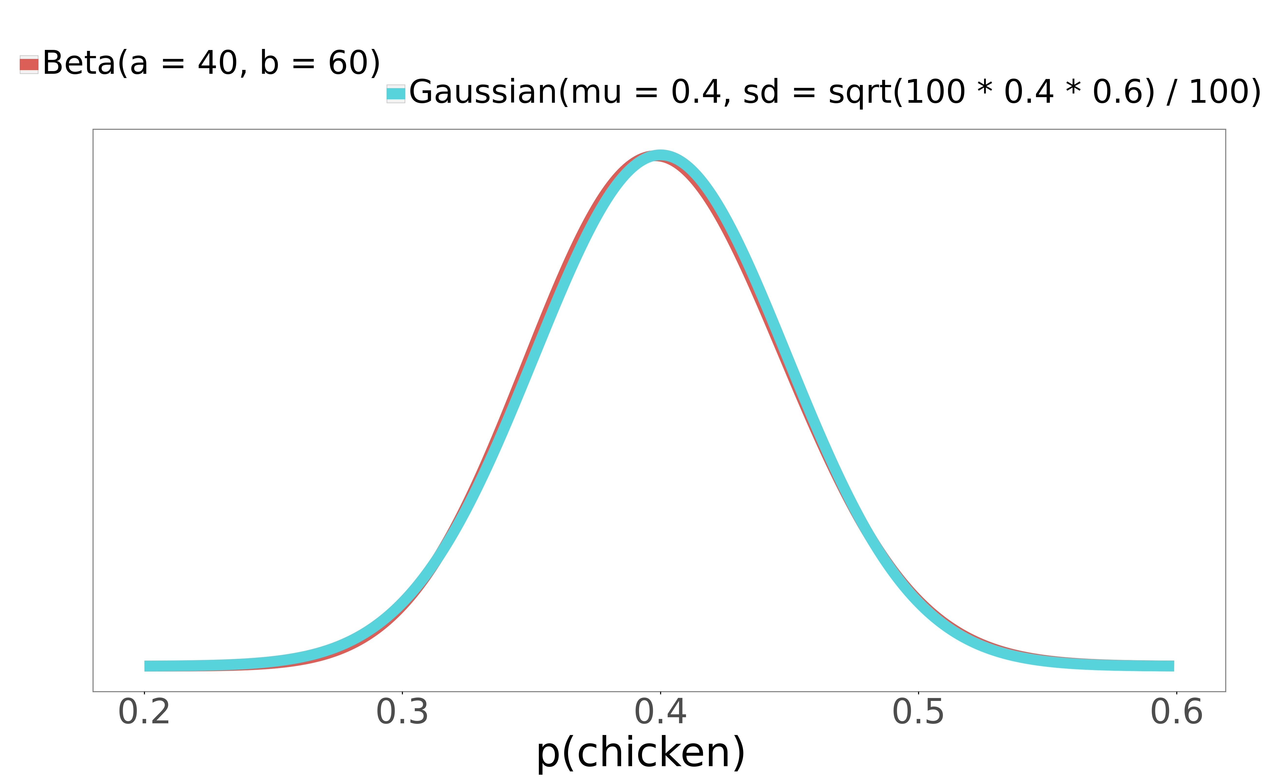
You work for a fancy restaurant. Fancy restaurants tend to have small menus. Your restaurant is extremely fancy, and thus has a 2-item menu: patrons can choose steak, or they can choose chicken. You want to compute the probability that a patron next week will order chicken, along with the uncertainty intervals around this probability. In the past week, 40 people got chicken, and 60 got steak. Here are the Gaussian and Beta distributions for $n=100$ and $p=0.40$:

The Gaussian approximation works very well here - it's nearly identical to the exact Beta solution. The 95% interval for the Beta is (0.307, 0.497), and the 95% interval for the Gaussian is (0.304, 0.496). For both, the mean is 0.40, like we'd expect. The uncertainty intervals tells us that from the experience of just 100 patrons, there's a 95% probability that between 30% and 50% of customers will order chicken next week. 

An example where the approximation breaks

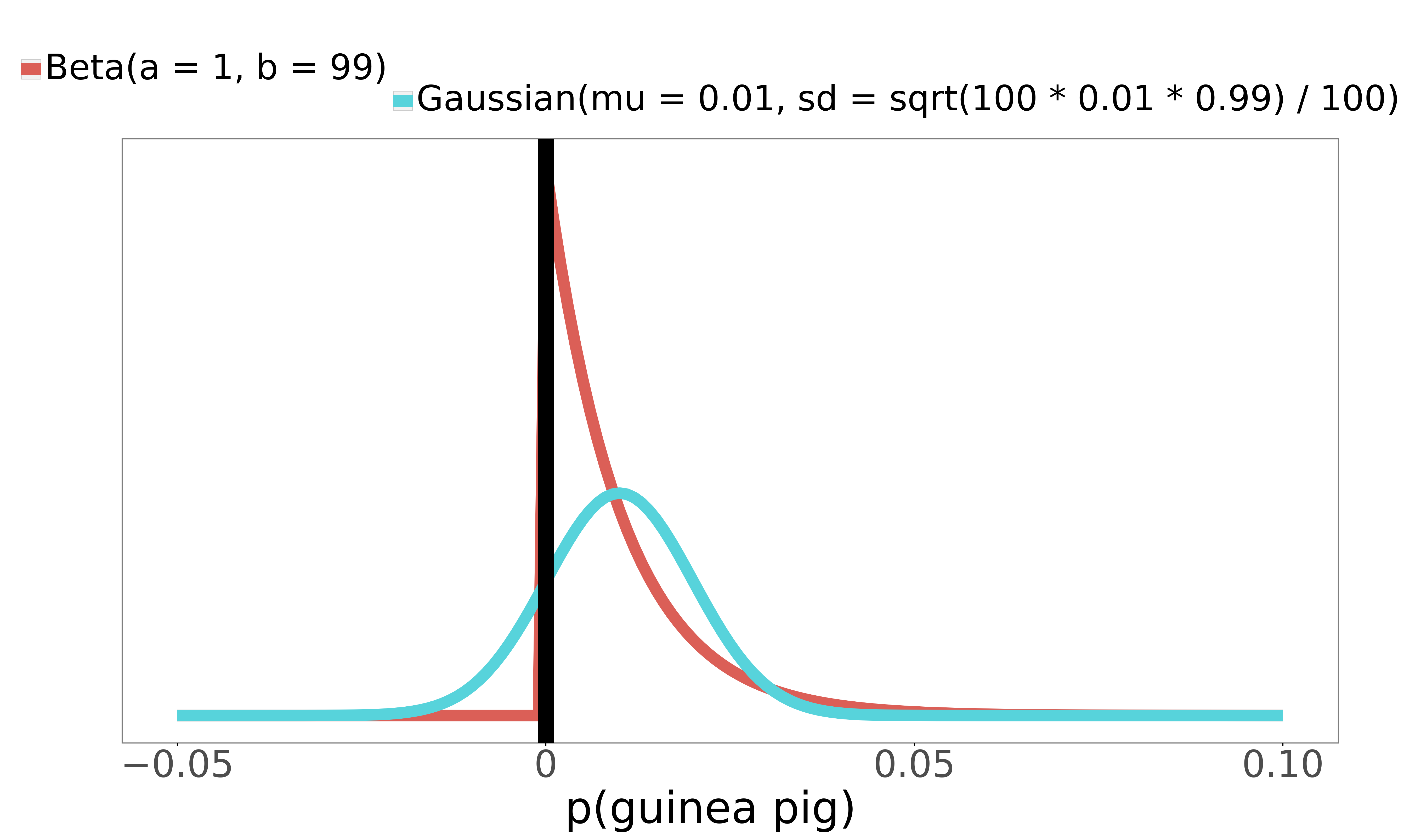
You're doing a test week where, instead of chicken, the restaurant serves guinea pig. So people can choose guinea pig or steak. Guinea pigs are seen as more like pets in the US, and also (from personal experience) just don't taste terribly good, so at the end of the week, only one adventurous soul has ordered it. 1 guinea pig, 99 steak. Check out the distributions:

I've marked 0 probability with a heavy black vertical line. The Gaussian approximation extends left of 0! The Gaussian 95% interval this time is [-0.01, 0.03] - a decent chunk of its mass is over negative probabilities. It says that there's a 95% probability that between -1% and 3% of patrons will order guinea pig next week. There is no sensible interpretation of these negative probabilities - the approximation has broken. Meanwhile, the Beta distribution has changed shape without issue, for a 95% interval of [0.0, 0.037]. Notice too how different the shape of this correct distribution is from the always-symmetrical Gaussian.

This comes up often

Computations from my own work where there was count data with small $n$ and small $p$:

• What is the probability that a patient who had a stent put into their heart will have a masectomy within 6 months?
• What proportion of surgeries at Regions hospital in the past two years were for the removal of cancerous thyroids?

In both of these projects, we had to compute probabilities like this for thousands of combinations of surgeries and hospitals, so we needed a procedure that didn't require eyeing distributions or doing hand modifications. The Beta was perfect; the Gaussian approximation would have broken.

Some made up examples where the Gaussian approximation would probably break, if you tried to use it to get uncertainty intervals:

• What is the probability of my car being stolen this year, using data from the 10-block radius around my house?
• What is the probability that, this year, I get sick as bad as I did in the summer of 2013?
• How often do local dog shelters offer up young wolves for adoption without realizing it?
• My logistic regression, when tested on an out-of-sample dataset of 50 data points, got all of them correct. What is the probability of misclassification on future data?
• I trained a gradient booster on a ton of data, and have a ton of out-of-sample data to analyze its accuracy on. However, I am particularly interested in how the model does on a key demographic: Minneapolis grandmothers with arthritis who frequent coffee shops. I only have 20 of these in my test set. My model misclassified 2 of them. What is the probability of misclassification on this type of grandma in future data?

There are many problems like this.

Code for the Beta distribution

Short and easy! Using the Gaussian is actually more work, because you have to remember or look up the formula for the standard deviation.

Python

from scipy.stats import beta
import numpy as np

chicken = 40
steak = 60
xs = np.arange(0, 1, 0.001)
beta_distribution = beta(chicken, steak)
beta_pdf = beta_distribution.pdf(xs)
beta_interval = beta_distribution.interval(0.95)

R

chicken <- 40
steak <- 60
xs <- seq(0, 1, 0.001)

beta_pdf = dbeta(xs, chicken, steak)
beta_interval = qbeta(c(0.025, 0.975), chicken, steak)

Super easy. 

 

Binary proportions like this come up all the time in data analysis. The Gaussian approximation became popular in a time before languages like R and Python, when computers were slow and people sometimes had to do these calculations by hand. With modern computers and statistical languages, using the Beta is easy, and gives you the exact answer every time. You don't even need to bother with thinking about and checking whether the Gaussian approximation is appropriate for your $p$ and $n$ - just use the Beta in every case, and be done with it.

2 comments

Comments sorted by top scores.