Interpreting Modular Addition in MLPs

post by Bart Bussmann (Stuckwork) · 2023-07-07T09:22:51.940Z · LW · GW · 0 comments

Contents

  Summary
  Background
  Training the Network
  Looking at Activations and Weights
  Interpretation
    1. Looking at Cosine Parameters
    2. Replacing Neuron Weights
    3. Randomly Initialized Cosine Neurons
  What do we learn from this?
  Open questions I'm thinking about
None
No comments

Summary

In this post, we investigate one of Neel Nanda's 200 Concrete Open Problems in Mechanistic Interpretability [LW · GW], namely problem A3.3: Interpret a 2L MLP (one hidden layer) trained to do modular addition.

The network seems to learn the following function:

$logit\left(c\right)\propto {\sum }_{i=0}^N\text{relu}\left(u_{1_i}\right(\cos (w_{i}a+s_{1_i})+\cos (w_{i}b+s_{2_i})\left)\right)\left(u_{2_i}\cos \right(w_{i}c+s_{1_i}+s_{2_i})+o_i)$

The code to reproduce the experiments in this post can be found here.

Background

In their paper, Progress Measures For Grokking Via Mechanistic Interpretability, Neel Nanda et. al find that the one-layer transformers learn a surprisingly funky algorithm for modular addition. Modular addition is the function $c=(a+b)\text{mod}P$, where P = 113 in both my and the original experiments.

In the original work, they find that a 1-layer Transformer learns an algorithm where the numbers are converted to frequencies with a memorized Discrete Fourier Transform, added using trig identities, and converted back to the answer.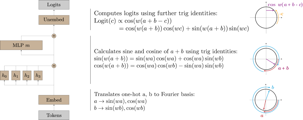

 

The goal of my project is to investigate whether a simple MLP with one hidden layer learns a similar algorithm, or something completely different.

Training the Network

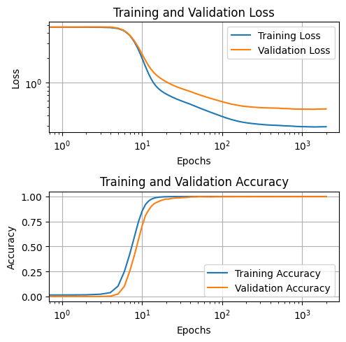
I create a dataset with all possible combinations of a and b, where a and b are integers in the range (0, 112). This gives me a dataset of 12769 samples, of which 80% is used for training and 20% for validation. The inputs and outputs are one-hot encoded, which means that the MLP has 226 input neurons and 113 output neurons. In the hidden layer, we use 100 neurons with ReLu activation^[1]. We use an AdamW optimizer with a learning rate of 0.003, batch size of 128, and weight decay of 0.5.^[2] We train the network for 2000 epochs, which is plenty to get near-perfect accuracy on both training and validation sets.

Looking at Activations and Weights

Now that the network is trained, let's take a look at the activations. We make a plot where we show the activation of some neurons for every possible value of a and b.

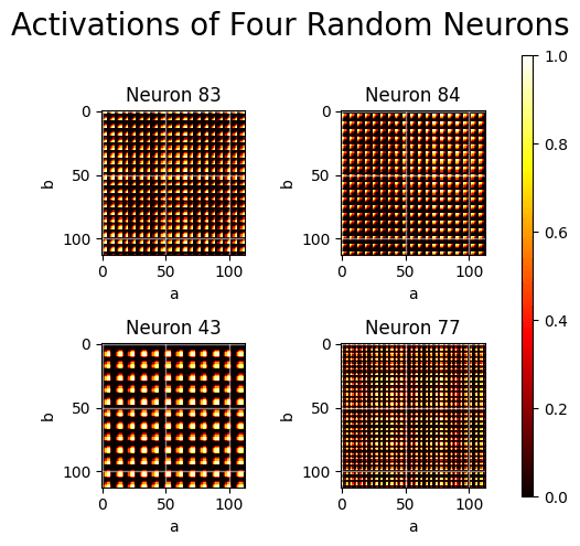
Oooh, pretty patterns! That must mean that the weights in the first layer are encoding the input in some periodic manner. Let's take a closer look at the input weights for Neuron 43, and see if they can be described by a sine/cosine function like the embedding layer in the previous work.

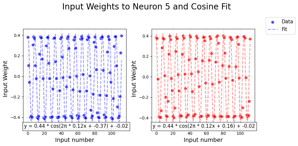
That looks like a great fit! Looking at the formulas of the fitted functions above (at the bottom of the plot), we observe that the weights coming from a and b follow a cosine function with the same scale, frequency, and offset, but with a different phase shift. Let's check if that's the case for all neurons.

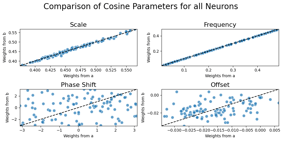
Interesting! The input weights from a and b to a particular neuron both follow cosine functions with the same scale and frequency. However, the fitted cosine functions from a and b typically have a different phase shift. The vertical offsets seem small for all learned functions, and I assume therefore unimportant. 

Concluding from this, the individual neurons in this MLP seem to be representing the following function: $\text{relu}(u_1\ast (\cos (w\ast a+s_1)+\cos (w\ast b+s_2)\left)\right)$.^[1]

Interpretation

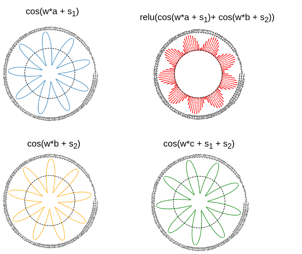
How can we interpret these neurons? Every neuron in the hidden layer activates strongly when input number a is in a certain period and b is in the same (but shifted) period. For example, a hidden neuron might activate when a is an even number and b is an uneven number. In this case, this neuron could be a detector for when the output c is an uneven number!

Can we generalize this? A neuron in the hidden layer activates strongly when both $\cos (w\ast a+s_1)$ and $\cos (w\ast b+s_2)$ are close to their peak values.  We know that if both functions peak, then a is a number in the set $a=\frac{2\pi k_1-s_1}{w}$ and $b=\frac{2\pi k_2-s_2}{w}$, and thus our outcome c is in the set of numbers $c=\frac{2\pi k_3-s_1-s_2}{w}$.  

This means, that we expect that if a hidden neuron has learned the relationship $\text{relu}(u_1\ast (\cos (w\ast a+s_1)+\cos (w\ast b+s_2)\left)\right)$,  then this should activate strongly whenever $\cos (w\ast c+s_1+s_2)$ is high. The network is learning neurons that activate strongly whenever our outcome c is in a certain period! And if we have a large enough number of frequencies and phase shifts, we can find out what the answer to the modular addition is.  

Another way to interpret this is that every neuron is learning an approximate modular function of the inputs. For instance, a particular neuron might activate strongly if$a\text{mod}5\approx 1$ and $b\text{mod}5\approx 2$. This neuron will then activate strongly for any c where $c\text{mod}5\approx 3$.  

So, altogether, I hypothesize the neural network learns to approximate the following function:

$logit\left(c\right)\propto {\sum }_{i=0}^N\text{relu}\left(u_{1_i}\right(\cos (w_{i}a+s_{1_i})+\cos (w_{i}b+s_{2_i})\left)\right)\left(u_{2_i}\cos \right(w_{i}c+s_{1_i}+s_{2_i})+o_i)$ , where N is the number of hidden neurons.

How can we test this hypothesis? We make a few predictions:

1. The output weights also follow a cosine function $u_3\ast \left(\cos \right(w_3\ast c+s_3)$) + o, where $w_3\approx w_1\approx w_2$ and $s_3\approx s_1+s_2$. 
2. We can replace the input and output weights of neurons with their cosine approximations without losing too much accuracy.
3. If the hidden layer is large enough, we can probably approximate modular addition without any learning, by initializing the input weights to $\cos (wa+s_1)$ and $\cos (wb+s_2)$ and the output weights to $\cos (wc+s_1+s_2)$ by taking some random $w$, $s_1$, and $s_2$.

1. Looking at Cosine Parameters

Let's fit a cosine to the output weights to check our first prediction. If we plot the fitted cosine parameters and compare them with the cosine parameter of the input weights of each neuron, we get the following graph:

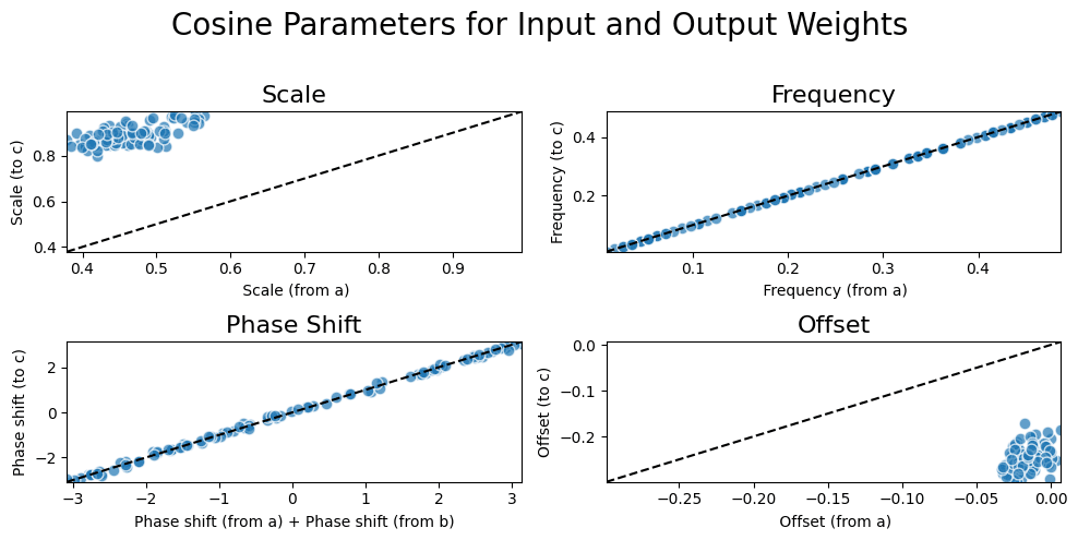
It's exactly what we predicted! The output weights of each neuron follow a cosine function with exactly the same frequency as the input weights, and indeed the phase shift is very close to the phase shift from the input weights from a and the input weights from b added together!

In other words, we confirm the following hypothesis: the output weights also follow a cosine function $u_2\ast \left(\cos \right(w_3\ast c+s_3)$) + o, where $w_3\approx w_1\approx w_2$ and $s_3\approx s_1+s_2$. 

2. Replacing Neuron Weights

We now know that if we fit a cosine function to the parameters, we get nice correspondences to the cosine functions of the input and output weights of the hidden neurons. However, we don't know how well the cosine fit actually represents the weights. 

In order to check this, we replace the input and output weights of a fraction of the neurons with their cosine approximations and check what the effect is on the performance.

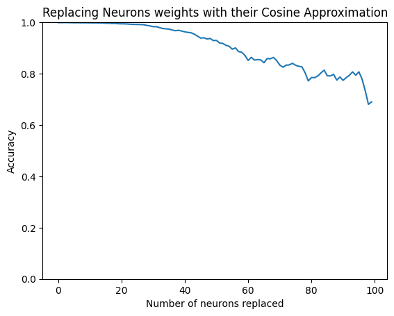
We can replace more than 90% of the neurons and still have an accuracy above 80%. So although the cosine approximations are not perfect representations of the weights, it seems to at least be a reasonable approximation of their function.

3. Randomly Initialized Cosine Neurons

In order to see whether$logit\left(c\right)\propto {\sum }_{i=0}^N\text{relu}\left(u_{1_i}\right(\cos (w_{i}a+s_{1_i})+\cos (w_{i}b+s_{2_i})\left)\right)\left(u_{2_i}\cos \right(w_{i}c+s_{1_i}+s_{2_i})+o_i)$ is indeed an algorithm that learns to do modular addition, it should in the limit of a large number of neurons converge to perfect accuracy, even if we sample random frequencies and phase shifts.

So, for N neurons we sample:

 $s_1\sim U_{[0,\pi ]}$,  

$s_2\sim U_{[0,\pi ]}$,

$k\sim U\{0,P\}$,

where $U_{[a,b]}$ is a continuous uniform distribution and $U\{a,b\}$ is a discrete uniform distribution. 

We set $w=\frac{2\pi k}{P}$, $u_1=0.5$,  $u_2=1$, and $o=0,$ and for every a and b, we calculate the logits and see if c indeed has the highest logit. 

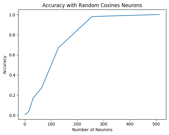
With 256 random neurons, we already have > 95% accuracy, and with 512 neurons we have perfect accuracy. This indicates that this algorithm is indeed a way to calculate modular addition. 

What do we learn from this?

•  MLPs with one hidden can learn modular addition. They do this by learning a cosine function over input and output weights for each neuron, where the cosine functions of the input and output weights share characteristics (frequency and phase shifts).
• The learned algorithm basically learns a set of modular functions of the inputs that detect when both inputs are in a certain period.
• Whereas the Transformer models from the previous work learn to embed the inputs in a few specific cosine frequencies, the one-layer MLP seems to favor (and probably needs) a broad range of cosine frequencies.

Open questions I'm thinking about

• This algorithm only works because of the one-hot encoding [LW · GW] that the model uses for the input and output. Can an MLP also grok modular addition if you use continuous inputs and outputs?  What algorithm does it learn then?
• What would be needed to automate this analysis? Could we use something like symbolic regression to automatically find this functional form? 
• In this network, the output weights of a hidden neuron are predictable from the input weights (up to a vertical offset and scale). Is this true in deeper models? What would this indicate? 

Thanks to Justis Mills for feedback on this post.
 

1. ^{^}

   The ReLu activation is just $f\left(x\right)=max(0,x)$, so it clips all negative numbers to 0 and is the most commonly used activation function in MLPs. 

2. ^{^}

   I didn't tune these hyperparameters much, and suspect the results are pretty robust to other hyperparameters (but didn't test this!)

0 comments

Comments sorted by top scores.