Causal Inference Sequence Part II: Graphical Models

post by Anders_H · 2014-08-04T23:10:02.285Z · LW · GW · Legacy · 4 comments

Contents

  Saturated and Unsaturated Models
  Statistical DAGs
  DAG Factorization
  D-Separation
  The Rules of D-Separation
  Faithfulness
  Causal DAGs
None
4 comments

(Part 2 of a Sequence on Applied Causal Inference. Follow-up to Part 1)

Saturated and Unsaturated Models

A model is a restriction on the possible states of the world: By specifying a model, you make a claim that you have knowledge about what the world does not look like.  

To illustrate this, if you have two binary predictors A and B, there are four groups defined by A and B, and four different values of E[Y|A,B].  Therefore, the regression E[Y|A,B] = β₀ + β₁*A  + β₂*B + β₃ * A * B  is not a real model :  There are four parameters and four values of E[Y|A,B], so the regression is saturated. In other words, the regression does not make any assumptions about the joint distribution of A, B and Y.   Running this regression in statistical software will simply give you exactly the same estimates as you would have obtained if you manually looked in each of the four groups defined by A and B, and estimated the mean of Y.

If we instead fit the regression model E[Y|A,B] = β₀ + β₁*A  + β₂*B , we are making an assumption: We are assuming that there is no interaction between A and B on the average value of Y.  In contrast to the previous regression, this is a true model:   It makes the assumption that the value of β₃ is 0.  In other words, we are saying that the data did not come from a distribution where β₃ is not equal to 0. If this assumption is not true, the model is wrong:  We would have excluded the true state of the world

In general, whenever you use models, think first about what the saturated model looks like, and then add assumptions by asking what parameters  you can reasonably assume are equal to a specific value (such as zero). The same type of logic applies to graphical models such as directed acyclic graphs (DAGs).  

We will talk about two types of DAGs:   Statistical DAGs are models for the joint distribution of the variables on the graph, whereas Causal DAGs are a special class of DAGs which can be used as models for the data generating mechanism.  

Statistical DAGs

A Statistical DAG is a graph that allows you to encode modelling assumptions about the joint distribution of the individual variables. These graphs do not necessarily have any causal interpretation.  

On a Statistical DAG, we represent modelling assumptions by missing arrows. Those missing arrows define the DAG in the same way that the missing term for β₃ defines the regression model above.  If there is a directed arrow between any two variables on the graph, the DAG is saturated or complete.  Complete DAGs make no modelling assumptions about the relationship between the variables, in the same way that a saturated regression model makes no modelling assumptions. 

DAG Factorization

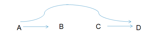
The arrows on DAGs are statements about how the joint distribution factorizes. To illustrate, consider the following complete DAG (where each individual patient in our study represents a realization of the joint distribution of the variables A, B, C and D.  ):

 

 

 

 Any joint distribution of A,B,C and D can be factorized algebraically according to the laws of probability as  f(A,B,C,D) = f(D|C,B,A) * f(C|B,A) * f(B|A) * f(A).   This factorization is always true, it does not require any assumptions about independence.  By drawing a complete DAG, we are saying that we are not willing to make any further assumptions about how the distribution factorizes.  

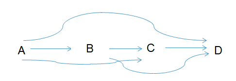
Assumptions are represented by missing arrows: Every variable is assumed to be independent of the past, given its parents.  Now, consider the following DAG with three missing arrows:

 

 

 

 

 This DAG is defined by the assumption that C is independent of the joint distribution of A and B, and that D is independent B, given A and C.   If this assumption is true, the distribution can be factorized as f(A,B,C,D) = f(D|C, A) * f(C) * f(B|A) * f(A).    Unlike the factorization of the complete DAG, the above is not a tautology. It is the algebraic representation of the independence assumption that is represented by the missing arrows. The factorization is the modelling assumption:  When arrows are missing, you are really saying that you have a priori knowledge about how the distribution factorizes. 

 

D-Separation

When we make assumptions such as the ones that define a DAG, other independences may automatically follow as logical implications. The reason DAGs are useful, is that you can use the graphs as a tool for reasoning about what independence statements are logical implications of the modelling assumptions. You could reason about this using algebra, but it is usually much harder.  D-Separation is a simple graphical criterion that gives you an immediate answer to whether a particular statement about independence is a logical implication of the independences that define your model.

Two variables are independent (in all distributions that are consistent with the DAG) if there is no open path between them.  This is called «d-separation».  D-Separation is useful because it allows us to determine if a particular independence statement is true within our model.   For example, if we want to know if A is independent of B given C, we check if A is d-separated from B on the graph where C is conditioned on

A path between A and B is any set of edges that connect the two variables. For determining whether a path exists, the direction of the arrows does not matter:  A-->B-->C and A-->B<--C are both examples of paths between A and C.    Using the rules of D-separation, you can determine whether paths are open or closed.  

 

The Rules of D-Separation

Colliders:

If you are considering three variables, they can be connected in four different ways:

 A --> B --> C

 A <-- B <-- C

 A <-- B --> C

 A --> B <-- C

 

• In the first three cases, B is a non-collider.
• In the fourth case,  B is a collider: The arrows from A and C "collide" in B.
• Non-Colliders are (normally) open, whereas colliders are (normally) closed
• Colliders are defined relative to a specific pathway.  B could be a collider on one pathway, and a non-collider on another pathway 

 

Conditioning:

If we compare individuals within levels of a covariate, that covariate is conditioned on.  In an empirical study, this can happen either by design, or by accident. On a graph, we represent “conditioning” by drawing a box around that variable.  This is equivalent to introducing the variable behind the conditioning sign in the algebraic notation

 

• If a non-collider is conditioned on, it becomes closed.
• If a collider is conditioned on, it is opened.
• If the descendent of a collider is conditioned on, the collider is opened

 

Open and Closed Paths:

 

• A path is open if and only if all variables on the path are open. 
• Two variables are D-separated if and only if there is no open path between them
• Two variables are D-separated conditional on a third variable if and only if there is no open path between them on a graph where the third variable has been conditioned on.

 

Colliders:

Many students who first encounter D-separation are confused about why conditioning on a collider opens it.  Pearl uses the following thought experiment to illustrate what is going on:

Imagine you live in a world where there is a sprinkler that sometimes randomly turns on, regardless of the weather. In this world, whether the sprinkler is on is independent of rain:  If you notice that the sprinkler is on, this gives you no information about whether it rains. 

However, if the sprinkler is on, it will cause the grass to be wet. The same thing happens if it rains. Therefore, the grass being wet is a collider.   Now imagine that you have noticed that the grass is wet.  You also notice that the sprinkler is turned "off".  In this situation, because you have conditioned on the grass being wet,  the fact that the sprinkler is off allows you to conclude that it is probably raining.  

Faithfulness

D-Separation says that if there is no open pathway between two variables, those variables are independent (in all distributions that factorize according to the DAG, ie, in all distributions where the defining independences hold).  This immediately raises the question about whether the logic also runs in the opposite direction:  If there is an open pathway between two variables, does that mean that they are correlated?

The quick answer is that this does not hold, at least not without additional assumptions.   DAGs are defined by assumptions that are represented by the missing arrows:  Any joint distribution where those independences hold, can be represented by the DAG, even if there are additional independences that are not encoded.   However, we usually think about two variables as correlated if they are connected:  This assumption is called faithfulness

Causal DAGs

Causal DAGs are models for the data generating mechanism. The rules that apply to statistical DAGs - such as d-separation - are also valid for Causal DAGs.  If a DAG is «causal», we are simply making the following additional assumptions: 

• The variables are in temporal (causal) order
• If two variables on the DAG share a common cause, the common cause is also shown on the graph

If you are willing to make these assumptions, you can think of the Causal DAG as a map of the data generating mechanism. You can read the map as saying that all variables are generated by random processes with a deterministic component that depends only on the parents.  

For example,  if variable Y has two parents A and U, the model says that Y^a =  f(A, U, *) where * is a random error term.   The shape of the function f is left completely unspecified, hence the name "non-parametric structural equations model".   The primary assumption in the model is that the error terms on different variables are independent.  

You can also think informally of the arrows as the causal effect of one variable on another:  If we change the value of A, this change would propagate to downstream variables, but not to variables that are not downstream.

Recall that DAGs are useful for reasoning about independences.  Exchangeability assumptions are a special type of independence statements: They involve counterfactual variables.  Counterfactual variables belong in the data generating mechanism, therefore, to reason about them, we will need Causal DAGs.  

A simplified heuristic for thinking about Causal DAGs is as follows:   Correlation flows through any open pathway, but causation flows only in the forward direction.  If you are interested in estimating the causal effect of A on Y, you have to quantify the sum of all forward-going pathways from A to Y.   Any open pathway from A to Y which contains an arrow in the backwards direction will cause bias. 

In the next part in this sequence (which I hope to post next week), I will give a more detailed description of how we can use Causal DAGs to reason about bias in observational research, including confounding bias, selection bias and mismeasurement bias. 

(Feedback is greatly appreciated:  I invoke Crocker's rules.  The most important types of feedback will be if you notice anything that is wrong or misleading.  I also greatly appreciate feedback on whether the structure of the text works, whether the sentences are hard to parse and whether there is any background information that needs to be included)

4 comments

Comments sorted by top scores.