Open Source Replication & Commentary on Anthropic's Dictionary Learning Paper

post by Neel Nanda (neel-nanda-1) · 2023-10-23T22:38:33.951Z · LW · GW · 12 comments

Contents

  Introduction
  TLDR
  Features
    Exploring Neuron Sparsity
    Case Studies
  Ultra Low Frequency Features Are All The Same Feature
  Implementation Details
  Misc Questions
None
12 comments

This is the long-form version of a public comment on Anthropic's Towards Monosemanticity paper

Introduction

Anthropic recently put out a really cool paper about using Sparse Autoencoders (SAEs) to extract interpretable features from superposition in the MLP layer of a 1L language model. I think this is an awesome paper and I am excited about the potential of SAEs to be useful for mech interp more broadly, and to see how well they scale! This post documents a replication I did of their paper, along with some small explorations building on it, along with (scrappy!) training code and weights for some trained autoencoders.

See an accompanying colab tutorial to load the trained autoencoders, and a demo of how to interpret what the features do. 

TLDR

• The core results seem to replicate - I trained a sparse autoencoder on the MLP layer of an open source 1 layer GELU language model, and a significant fraction of the latent space features were interpretable
  • I open source two trained autoencoders, here’s a tutorial for how to use them, and how to interpret a feature. 
    • And a (very!) rough training codebase
  • I give some of the implementation details, and tips for training your own.
• I investigate how sparse the decoder weights are in the neuron basis and find that they’re highly distributed, with 4% well explained by a single neuron, 4% well explained by 2 to 10, and the remaining 92% dense. I find this pretty surprising! 
  • Kurtosis shows the neuron basis is still privileged.
• I exhibit some case studies of the features I found, like a title case feature, and an "and I" feature
• I didn’t find any dead features, but more than half of the features form an ultra-low frequency cluster (frequency less than 1e-4). Surprisingly, I find that this cluster is almost all the same feature (in terms of encoder weights, but not in terms of decoder weights). On one input 95% of these ultra rare features fired!
  • The same direction forms across random seeds, suggesting it's a true thing about the model and not just an autoencoder artifact
  • I failed to interpret what this shared direction was
  • I tried to fix the problem by training an autoencoder to be orthogonal to this direction but it still forms a ultra-low frequency cluster (which all cluster in a new direction)
• Should the encoder and decoder be tied? I find that, empirically, the decoder and encoder weights for each feature are moderately different, with median cosine sim of only 0.5, which is empirical evidence they're doing different things and should not be tied. 
  • Conceptually, the encoder and decoder are doing different things: the encoder is detecting, finding the optimal direction to project onto to detect the feature, minimising interference with other similar features, while the decoder is trying to represent the feature, and tries to approximate the “true” feature direction regardless of any interference.

Features

Exploring Neuron Sparsity

One of the things I find most interesting about this paper is the existence of non neuron basis aligned features. One of the big mysteries (by my lights) in mechanistic interpretability is what the non-linearities in MLP layers are actually doing, on an algorithmic level. I can reason about monosemantic GELU neurons fairly easily (like a French neuron) - essentially thinking of it as a soft ReLU, that collect pieces of evidence for the presence of a feature, and fire if they cross a certain threshold (given by the bias). This can maybe extend to thinking about a sparse linear combination of neurons (eg fewer than 10 constructively interfering to create a single feature). But I have no idea how to reason about things that are dense-ish in the neuron basis!

As a first step towards exploring this, I looked into how dense vs sparse each non-ultra-low frequency feature was. Conceptually, I expected many to be fairly neuron-sparse - both because I expected interpretable features to tend to be neuron sparse in general, and because of the autoencoder setup: on any given input a sparse set of neurons fire, so it seems that learning specific neurons/clusters of neurons is a useful dictionary feature. 

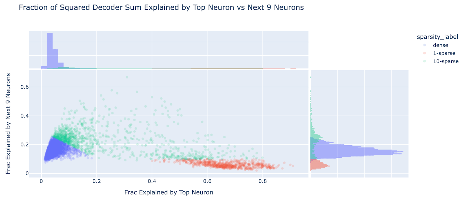
However, a significant majority of features seem to be fairly dense in the neuron basis! As a crude metric, for each dictionary feature, I took the sum of squared decoder weights, and looked at the fraction explained by the top neuron (to look for 1-sparse features), and by the next 9 neurons (to look for 10-ish-sparse features). I use decoder rather than encoder, as I expect the decoder is closer to the “true” feature direction (ie how it’s computed) while the encoder is the subtly different “optimal projection to detect the feature” which must account for interference. In the scatter plot below we can see 2-3 rough clusters - dense features near the origin (low on both metrics, which I define as fve_top_10<0.35), 1-sparse features (fve_top_1>0.35, fve_next_9<0.1), and 10-ish-sparse features (the diffuse mess of everything else). I find ~92.1% of features are dense, ~3.9% are 1-sparse and ~4.0% are 10-ish-sparse.

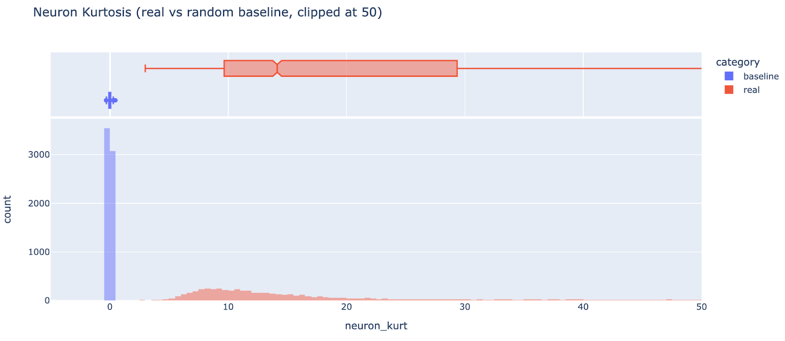
Another interesting metric is neuron kurtosis, ie taking the decoder weights for each feature (in the MLP neuron basis) and taking the kurtosis (metric inspired by this paper, and by ongoing work with Wes Gurnee). This measures how “privileged” the neuron basis is, and is another way to detect unusually neuron-sparse features - the (excess) kurtosis of a normal distribution is zero, and applying an arbitrary rotation makes everything normally distributed. We can clearly see in the figure below that the neuron basis is privileged for almost all features, even though most features don’t seem neuron-sparse (red are real features, blue is the kurtosis of a randomly generated normally distributed baseline. Note that the red tail goes up to 1700 but is clipped for visibility).

 

I haven’t studied whether there’s a link between level of neuron sparsity and interpretability, and I can’t rule out the hypothesis that autoencoders learn features with significant noise and that the “true” feature is far sparser. But this seems like evidence that being dense in the neuron basis is the norm, not the exception.

Case Studies

Anecdotally a randomly chosen feature was often interpretable, including some fairly neuron dense ones. I didn’t study this rigorously, but of the first 8 non-ultra-low features 6 seemed interpretable. From this sample, I found:

• A title case/headline feature, that was dominated by a single neuron and boosted the logits for tokens beginning with a capital or that come in the middle of words
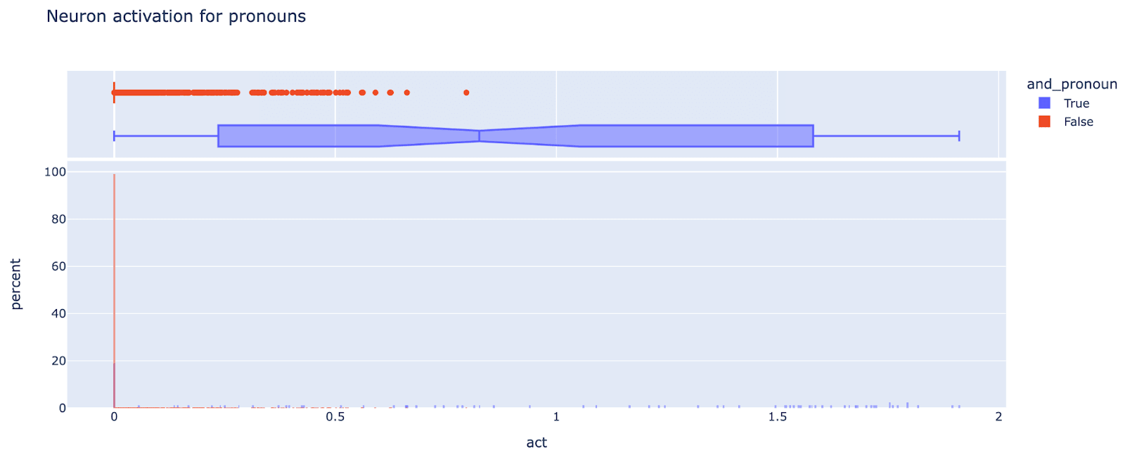
• A “connective followed by pronoun” feature that activated on text like “and I” and boosts the `‘ll` logit
  • 
• Some current token based features, eg one that activates on ` though` and one that activates on ` (“`
• A previous token based feature, that activates on the token after de/se/le (preference for ` de`)

Ultra Low Frequency Features Are All The Same Feature

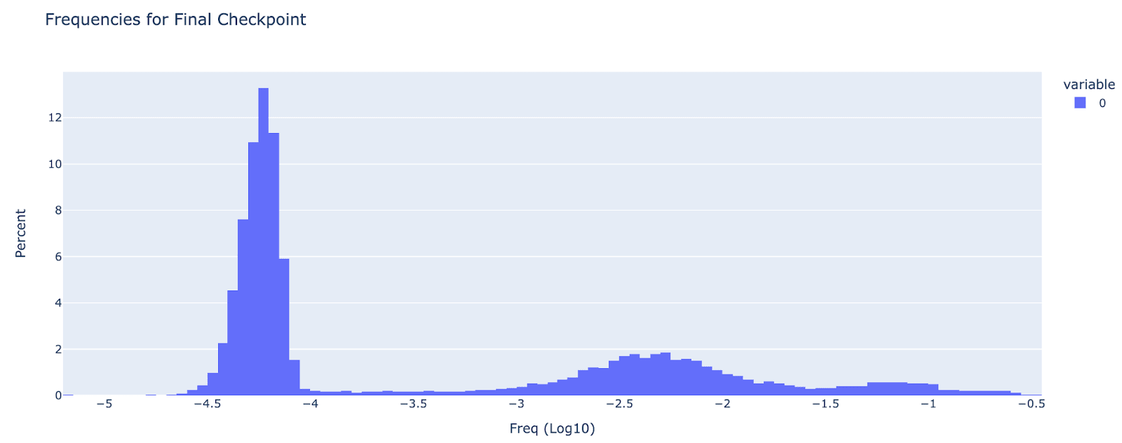
Existence of the ultra-low frequency cluster: I was able to replicate the paper’s finding of an ultra-low frequency cluster, but didn’t find any truly dead neurons. I define the ultra-low frequency cluster as anything with frequency less than 1e-4, and it is clearly bimodal, with about 60% of features as ultra-low frequency and 40% as normal. This is in contrast to 4% dead and 7% ultra-low in the A/1 autoencoder, I’m not sure of why there’s a discrepancy, though it may be because I resampled neurons with re-initialising weights rather than the complex scheme in the paper. Anecdotally, the ultra-low frequency features were not interpretable, and are not very important for autoencoder performance (reconstruction loss goes from 92% to 91%)

The encoder weights are all the same direction: Bizarrely, the ultra-low frequency entries in the dictionary are all the same direction. They have extremely high cosine sim with the mean (97.5% have cosine sim more than 0.95)

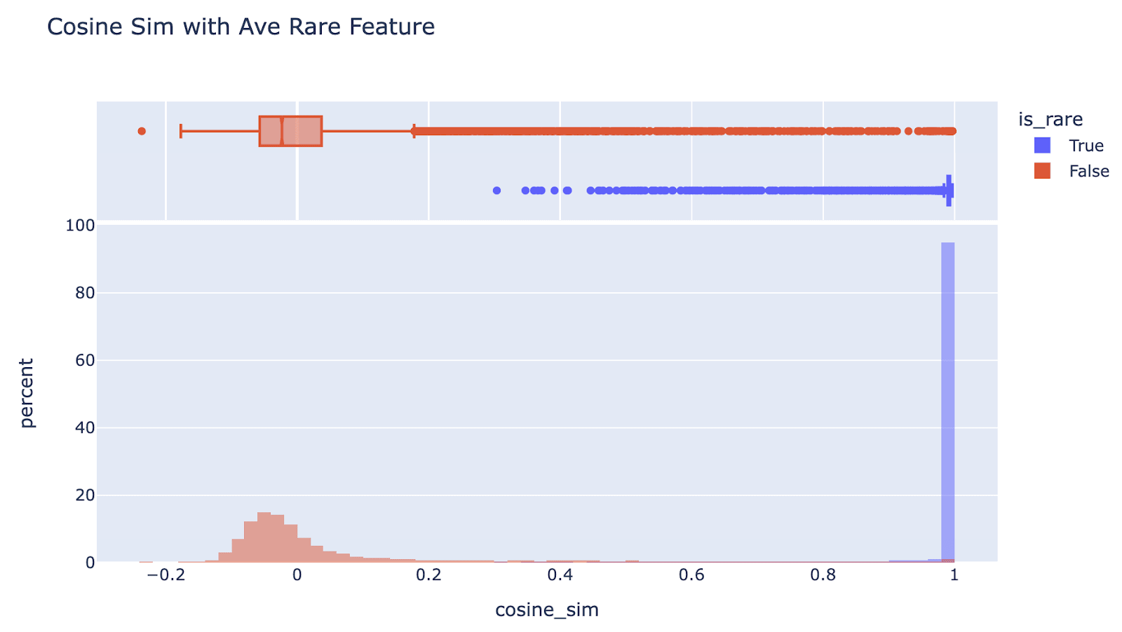
Though they vary in magnitude, as can be seen from their projection onto the mean direction (I’m not sure why this is bimodal). (Note that here I’m just thinking about |encoder|, and really |encoder| * |decoder| is the meaningful property, but that gets a similar distribution)

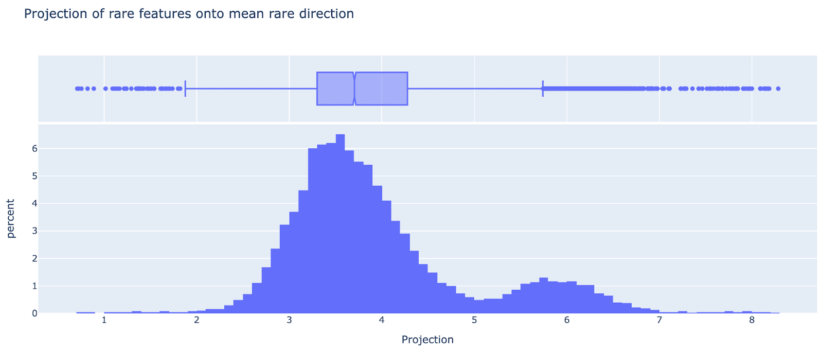
This means the ultra low features are highly correlated with each other, eg I found one data point that’s extreme in the mean direction where 95% of the ultra low features fired on it

The decoder weights are not all the same direction: On the other hand, the decoder weights seem all over the place! Very little of the variance is explained by a single direction. I’m pretty confused by what’s going on here. 

The encoder direction is consistent across random seeds: The natural question is whether this direction is a weird artefact of the autoencoder training process, or an actual property of the transformer. Surprisingly, training another autoencoder with a different random seed finds the same direction (cosine sim 0.96 between the means). The fact that it’s consistent across random seeds makes me guess it’s finding something true about the autoencoder.

What does the encoder direction mean? I’ve mostly tried and failed to figure out what this shared feature means. Things I’ve tried:

• Inspecting top dataset examples didn’t get much pattern, and it drops when seemingly non-semantic edits are made to the text. 
• It’s not sparse in the neuron basis
• It’s output weights aren’t sparse in the vocab basis (though correlates with “begins with a space)
• It’s nothing to do with the average MLP activation, or MLP activation singular vectors, or MLP acts being high norm

A sample of texts where the average feature fires highly:

Can we fix ultra-low frequency features? These features are consuming 60% of my autoencoder, so it’d be great if we could get rid of them! I tried the obvious idea of forcing the autoencoder weights to be orthogonal to this average ultra low feature direction at each time step, and training a new autoencoder. Sadly, this autoencoder had its own cluster of ultra-low frequency features, which also had significant cosine sims with each other, but a different direction. 

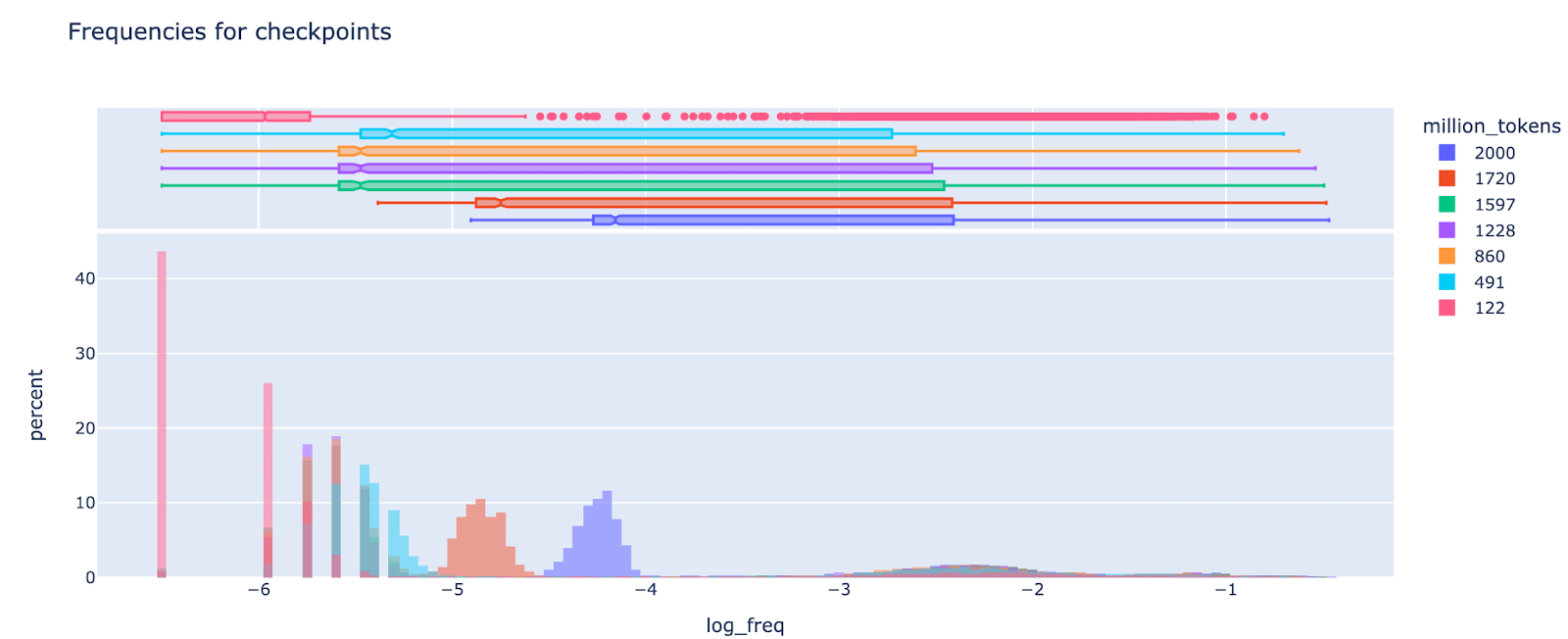
Phase transition in training for feature sparsity: Around 1.6B tokens, there was a seeming phase transition where ultra low density features started becoming more common. I was re-initialising the weights every 120M tokens for features of frequency less than 1e-5, but I found that around 1.6B (the 13th ish reset) they started to drift upwards in frequency, and at some point crossed the 1e-5 boundary (which broke my resetting code!). By 2B tokens they were mostly 1e-4.5 to 1e-4, still a distinct mode, but drifting upwards. It's a bit hard to tell, but I don't think  there was a constant upward drift, it seems to only happen in late training, based on inspecting checkpoints

(Figure note: the spike at -6.5 corresponds to features that never fire)

Implementation Details

• The model was gelu-1l, available via the TransformerLens library. It has 1 layer, d_model = 512, 2048 neurons and GELU activations. It was trained on 22B tokens, a mix of 80% web text (C4) and 20% Python code
• The autoencoders trained in about 12 hours on a single A6000 on 2B tokens. They have 16384 features, and L1 regularisation of 3e-3
  • The reconstruction loss (loss when replacing the MLP layer by the reconstruction via the autoencoder) continued to improve throughout training, and got to 92% (compared to zero ablating the MLP layer).
    • For context, mean ablation gets 25%
• Getting it working:
  • My first few autoencoders failed as L1 regularisation was too high, this showed up as almost all features being dead
  • When prototyping and training, I found it useful to regularly compute the following metrics:
    • The autoencoder loss (when reconstructing the MLP acts)
    • The reconstruction loss (when replacing the MLP acts with the reconstructed acts, and looking at the damage to next token prediction loss)
    • Feature frequency (including the fraction of dead neurons), both plotting histograms, and crude measures like “frac features with frequency < 1e-5” or 1e-4
  • I implemented neuron resampling, with two variations:
    • I resampled any feature with frequency < 1e-5, as I didn’t have many truly dead features, and the ultra-low frequency features seemed uninterpretable - this does have the problem of preventing my setup from learning true ultra-low features though. 
    • I took the lazy route of just re-initialising the weights
  • I lacked the storage space to easily precompute, shuffle and store neuron activations for all 2B tokens. I instead maintained a buffer of acts from 1.5M prompts of 128 tokens each, shuffled these and then took autoencoder training batches from it (of batch size 4096). When the buffer was half empty, I refilled it with new prompts and reshuffled. 
    • I was advised by the authors that it was important to minimise autoencoder batches having tokens from the same prompt, this mostly achieved that though tokens from the same prompt would be in nearby autoencoder batches, which may still be bad. 
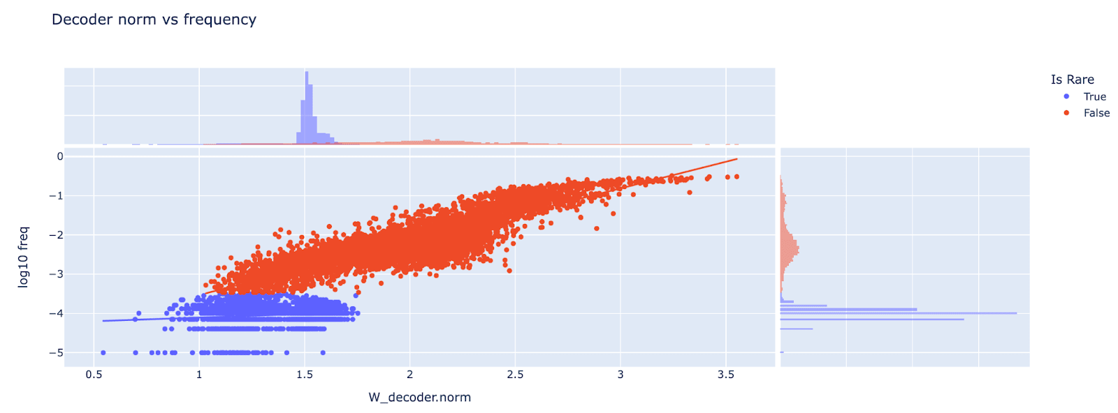
• Bug: I failed to properly fix the decoder to be norm 1. I removed the gradients parallel to the vector, but did not also reset the norm to be norm 1. This resulted in a decoder norm with some real signal, and may have affected my other results
  • 

Misc Questions

Should encoder and decoder weights be tied? In this paper, the encoder and decoder weights are untied, while in Cunningham et al they’re tied (tied meaning W_dec = W_enc.T). I agree with the argument given in this paper that, conceptually, the encoder and decoder are doing different things and should not be tied. I trained my autoencoders with untied encoder and decoder.

My intuition is that, for each feature, there’s a “representation” direction (its contribution when present) and a “detection” direction (what we project onto to recover that feature’s coefficient). There’s a sparse set of active features, and we expect the MLP activations to be well approximated by a sparse linear combination of these features and their representation direction - this is represented by the decoder. To extract a feature’s coefficient, we need to project onto some direction, the detection direction (represented by the encoder). Naively, this is equal to representation direction (intuitively, the dual of the vector). But this only makes sense if all representation directions are orthogonal! We otherwise get interference from features with non-zero cosine sim between representations, and the optimal detection direction is plausibly different. Superposition implies more directions than dimensions, so they can’t all be orthogonal!

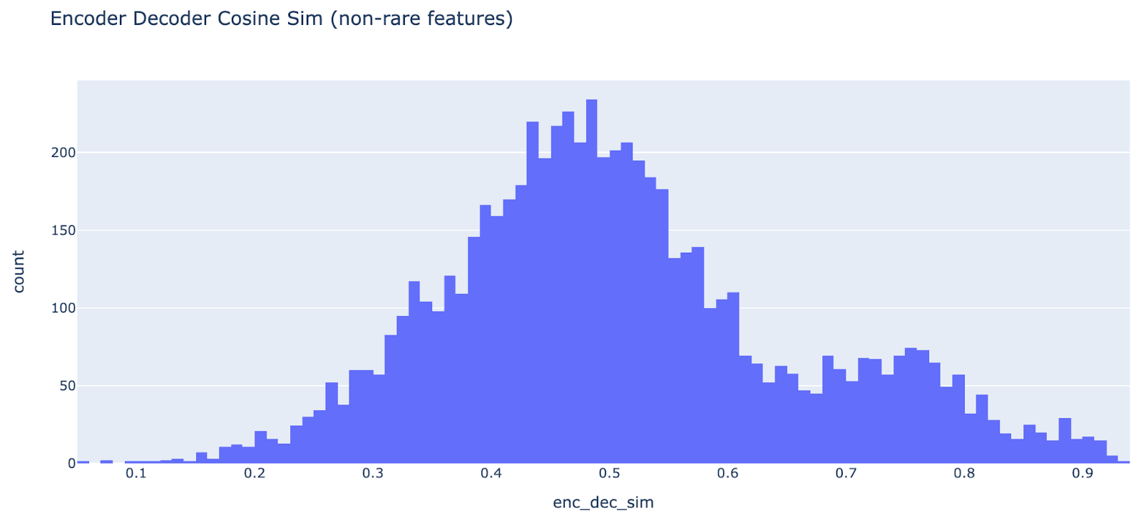
As some empirical evidence, we can check whether in practice the autoencoder “wants” to be tied by looking at the cosine sim between each feature’s encoder and decoder weights. The median (of non ultra low features) is 0.5! There’s some real correlation, but the autoencoder seems to prefer to have them not be equal. It also seems slightly bimodal (a big mode centered at 0.5 and one at 0.75 ish), I’m not sure why.

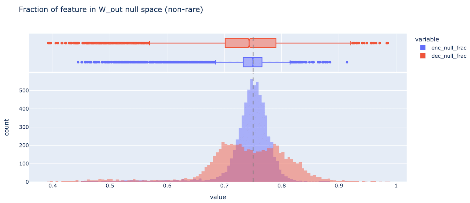
Should we train autoencoders on the MLP output? One weird property of transformers is that the number of MLP neurons is normally significantly larger than the number of residual stream dimensions (2048 neurons, 512 residual dims for this model). This means that 75% of the MLP activation dimensions are in the nullspace of W_out (the output weights of the MLP layer, ie the down-projection) and so cannot matter causally for the model. 

Intuitively, this means that a lot of the autoencoder’s capacity is wasted, representing the part of the MLP activations that doesn’t matter causally. A natural idea is to instead train the autoencoder on the MLP output (after applying W_out). This would get an autoencoder that’s 4x smaller and takes 4x less compute to run (for small autoencoders the cost of running the model dominates, but this may change for a very wide autoencoder). My guess is that W_out isn’t going to substantially change the features present in the MLP activations, but that training SAEs on the MLP output is likely a good idea (I sadly only thought of this after training my SAEs!)

Unsurprisingly, a significant fraction of each encoder and decoder weight is representing things in the null-space of W_out. Note that it’s significantly higher variance and heavier tailed than it would be for a random 512 dimensional subspace (a random baseline has mean 0.75 and std 0.013), suggesting that W_out is privileged (as is intuitive). 

 

12 comments

Comments sorted by top scores.