A short project on Mamba: grokking & interpretability

post by Alejandro Tlaie (alejandro-tlaie-boria) · 2024-10-18T16:59:45.314Z · LW · GW · 0 comments

Contents

  Executive summary
  Introduction
  A simple-yet-interesting enough task
  A minimalistic implementation of the SSM layer
  Differences with the original Mamba model
  Results
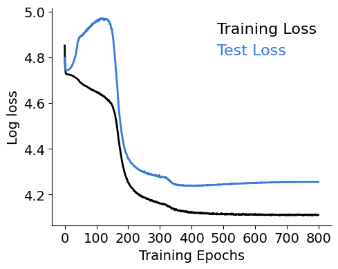
    It groks!
  A low-dimensional linear decomposition of the gating can be suggestive of learning
  Decomposing the tensor of gating activations reveals input parity
  Those factors extracted with the tensor decomposition are more directly related to learning and grokking
  Future work
None
No comments

Epistemic status: I've worked on this project for ~20h, on my free time and using only a Colab notebook.

Executive summary

I trained a minimalistic implementation of Mamba (details below) on the modular addition task. I found that:

1. This non-transformer-based model can also exhibit grokking (i.e., the model learns to generalise after overfitting to the training data).
2. There are tools that we can import from neuroscience that can help us interpret how the network representation changes as grokking takes place over training epochs.

Introduction

Almost all of the Mechanistic Interpretability (MI) efforts I've seen people excited about and the great majority of the techniques I've learned are related to Transformer-based architectures. At the same time, a competitive alternative (Mamba) was recently introduced and later scaled. To me, when coupling these two facts together, a giant gap between capabilities and safety emerges.

Thus, I think Mamba provides an interesting use case where we can test whether the more conceptual foundations of MI are solid (i.e., somewhat model-agnostic) and, therefore, whether MI can potentially survive another transformer-like paradigm shift on the race towards AGI.

For a bit more of context, Mamba is based on a special version of State Space Models (SSMs): add another S (for Structured) and you have one of its essential components. The actual architecture is slightly more complex, as you can see in this awesome post, than the S-SSM layer, but for this project I wrote up a minimal implementation that could get the job done.

A simple-yet-interesting enough task

The task that the model has to solve is: given two input integers ($x$ and $y$), return whether their sum is divisible by a big prime number ($p=113$, in this case). This is mapped into a setup that Autoregressive token predictors can deal with: one input example would consist of three tokens: '$x$', '$y$' and '$=$', and the only output token would be either '$0$' (if $(x+y)$ mod $p$ $\ne 0$) or '$1$' (otherwise).

My main reason for choosing this oddly specific task was that it's probably the most well understood and reversed engineered example using MI and simple transformers. In other words, I didn't have to re-invent the wheel.

A minimalistic implementation of the SSM layer

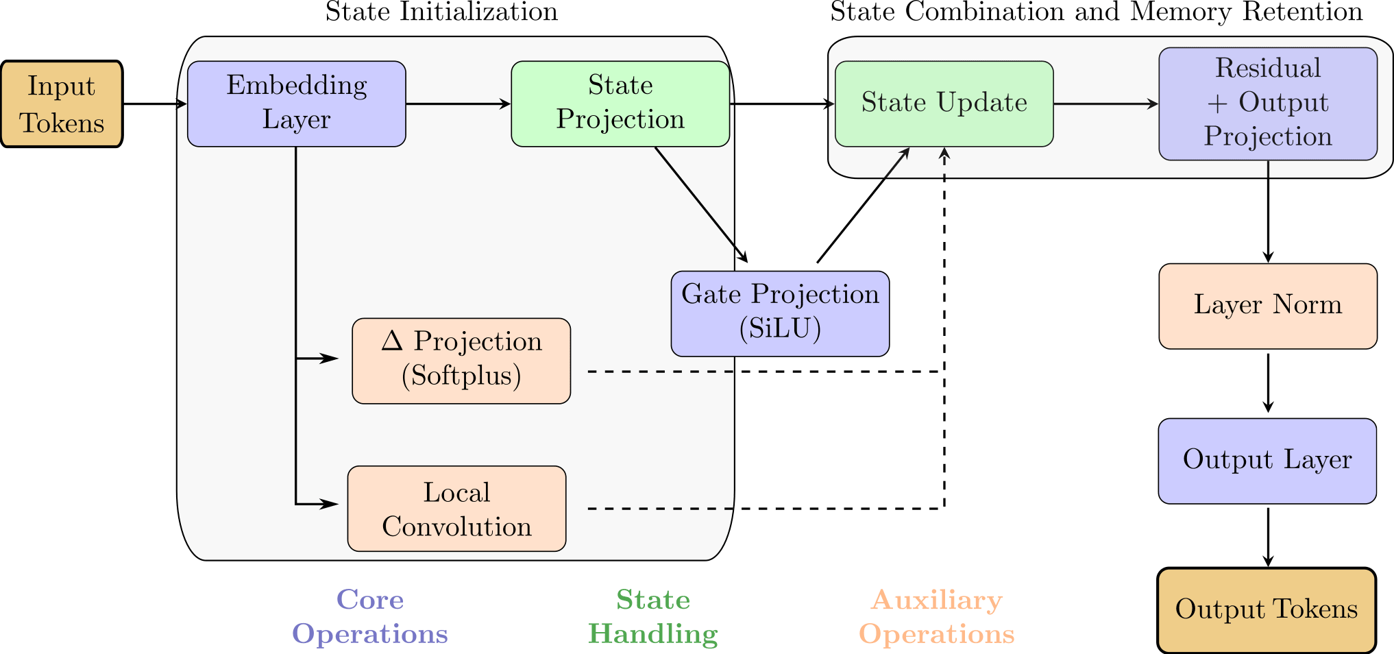
My MinimalMambaSSM implementation is a simplified version of the Mamba architecture, combining state-space modelling with gated recurrent mechanisms for efficient sequence learning. Its core components are:

1. Embedding layer: Transforms input tokens into dense vector representations of size d_model.

2. State projection and initialisation: Projects input representations to match internal state size and initialises a shared learnable state.

3. Gate and $\Delta$ projections: The gating mechanism mixes the current input with the previous state, using SiLU activation. The $\Delta$ projection modulates the state update with softplus activation.

4. Convolution for local mixing: A convolutional layer mixes local input features, capturing neighborhood interactions for richer state updates.

5. State update: The state is updated based on the gate, local mixing, and input projection, balancing between memory retention and new information integration.

6. Residual connection and output projection: Adds a residual connection from the last token, followed by an output projection and layer normalization for stabilization and efficient training.

7. Output layer: Projects the final representation to produce the model output.

Differences with the original Mamba model

This minimal implementation of the Mamba architecture significantly simplifies the original model. Concretely, here's how they differ:

1. Simplified layers: My minimal version uses fewer operations, reducing complexity by removing some of the auxiliary functions like additional convolutions or stacking layers.

2. Reduced state dynamics: The full Mamba architecture contains multiple SSM blocks and a detailed gating mechanism to manage state transitions over tokens. My minimal version only includes a single state update step, lacking the intricacies of dynamic SSM state mixing across layers.

3. Layer connectivity: The original Mamba architecture involves both SSM and convolutional layers for token mixing, designed to manage both local and global dependencies. In my minimal implementation, only a single convolution step is retained.

4. Depth of processing: The Mamba model is designed to capture long-range dependencies through multiple blocks stacked with residual connections. My minimal version retains only one such residual connection.

5. Modular flexibility: The Mamba block contains separate mixing pathways for both local (via convolutions) and long-term dependencies (via SSM states). My minimal implementation incorporates a straightforward gate and state projection, lacking multiple pathways.

So, in short, my minimal version aims to capture the essence of the Mamba architecture (mainly state management and gating) but doesn't have the depth and modular flexibility necessary to handle complex dependencies and large-scale data processing (i.e., it's suited for the simple task that I'm interested in).

Results

It groks!

I find this result interesting per se, I wasn't sure if grokking was a transformer's thing only!

Now, I wondered, what can I do on my toy model to interpret how this comes about? I think the key interpretable part of the model is within the gating mechanism. The majority of its expressivity comes from this, as it modulates how much to remember about the previous state and how much to simply look at the current state. In an extremely cool paper, the authors found that this mechanism is very closely related to gating in RNNs and to attention layers in transformers.

A low-dimensional linear decomposition of the gating can be suggestive of learning

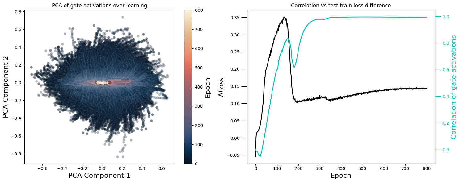
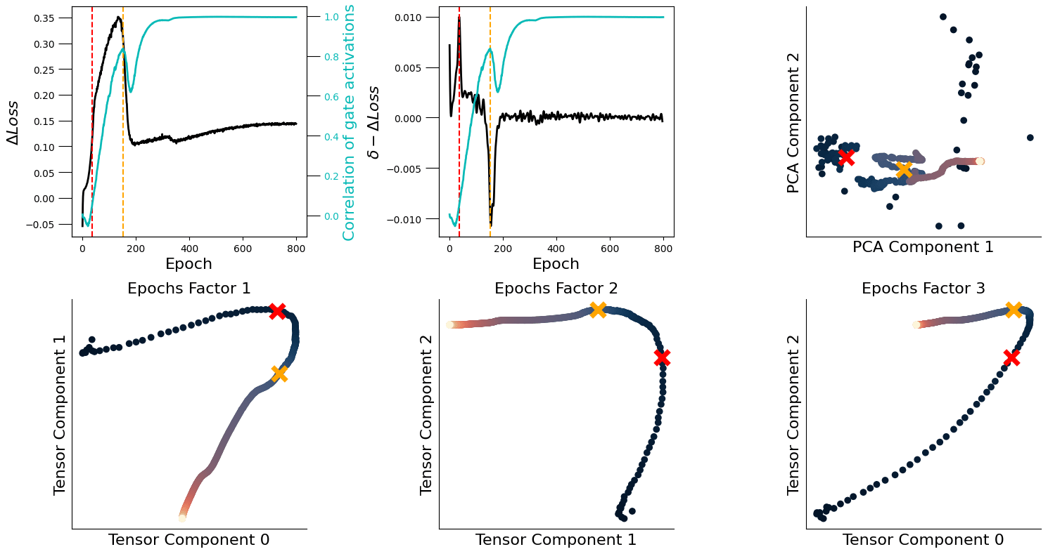
Thus, the matrix of gating activations is the central object I focused on. Particularly, I ended up with a $4D$ tensor of shape $(n_{samples},n_{epochs},n_{tokens},n_{gate})$. And, consequently, the first thing I did was to aggregate (averaging) activations over the token dimension and, for each epoch, compute the $2D$ PCA of the $(n_{samples},n_{gate})$ matrix. That is what you see on the left plot (the one that looks like a flipped Sauron eye).

This plot speaks to the fact that, at the beginning of the training process, all gate activations are basically randomly initialised (uncorrelated) and, as grokking happens, they collapse into a highly synchronous mode (which is the cyan line I plot at the right, together with the loss diference ($\Delta L=L_{test}-L_{train}$).

I was curious to see whether these simple PCs were already interpretable in some way, so I tried to relate them with $\Delta L$. To do that, I found special points along that curve: where its derivative is maximum (red line) and where it's minimum (orange line) —see the central plot. Then, I plotted $PC2$ against $PC1$ for each epoch (having previously computed the median over the $samples$ dimension) — see the rightmost plot:

I couldn't find any easily interpretable point in these trajectories, so I took a step back and thought: should I expect to find something special at the gate activations at all? To answer this question in the most obvious way I could think of, I plotted them at the selected epochs, and saw a confirmation of what I suspected:

As learning/grokking takes place, the activations over samples get more and more synchronised. However, also note that there is an activation specialisation, by which each gate dimension gets separated from the others and, thus, they are able to span more values (potentially, to represent the input in a richer way).

Coming back to my inability to extract information from the PCA decomposition, the key question was: why am I decomposing the $2D$ matrix $((n_{samples},n_{gate}))$? That is, having a background in computational neuroscience, I was aware that I could also directly decompose $3D$ tensor of shape $(n_{epochs},n_{tokens},n_{gate})$, so that I could extract factors on each of those dimensions.

Decomposing the tensor of gating activations reveals input parity

So, I did exactly that. Using tensortools, I computed the Canonical Polyadic decomposition (see here for a more intuitive explanation, if interested).

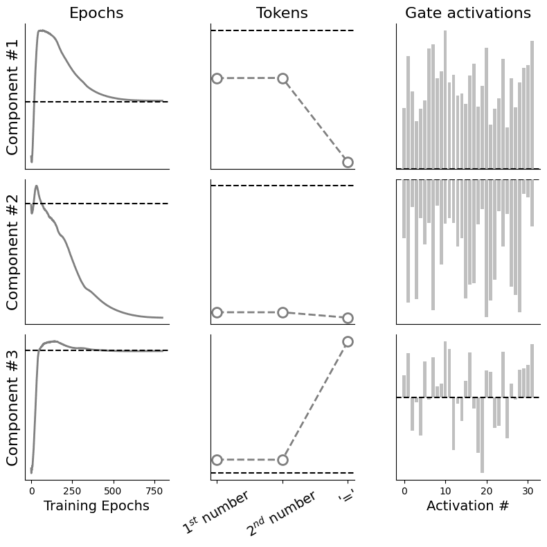
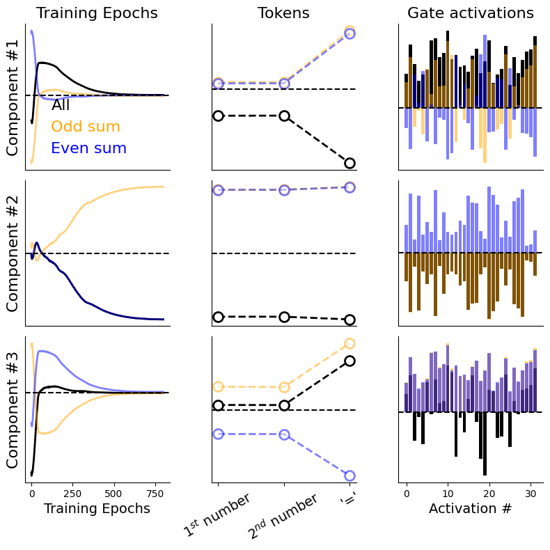
As there are some parts of this figure that may not be completely intuitive for everyone, let's begin by explaining the layout: each column shows a different factor —you can think of these as the latent variables that explain variance of the original tensor in a given direction; each row shows a different component —exactly in the same way as in PCA you have $PC1$, $PC2$, etc. I have also removed all y-labels for convenience (we're mainly interested in relative differences here) and I show where the $0$ is, as a dashed black horizontal line. Okay, now, to the actual plots.

For the epochs factor: the $1^{st}$ component seems to be closely tracking $\Delta L$. For the tokens factor: there is a symmetry by which the '$=$' token is disproportionately represented either positively ($3^{rd}$ component) or negatively ($1^{st}$ component); the two input numbers are symmetrically non-salient. For the gate factor: components $1$ and $2$ show clearly segmented and specialised gating patterns, whereas the third one exhibits a more mixed behavior.

I was curious to check whether one could go one step further and inspect whether these factors reflect anything regarding parity of the $x$, $y$ sum; my reasoning was that even numbers will never be divisible by a prime (except, of course, for $p\in \{1,2\}$) and, thus, they could probably be encoded differently. To check that hypothesis out, I re-computed the tensor decomposition in the exact same way as before but, before averaging over the $samples$ dimension, I split over those positions with the aforementioned parity:

What I show here is basically the same layout as before (the previously grey plot is now black, for better visibility) but I also now show the decompositions that correspond to both the odd and the even sums. Surprisingly (to me, I don't know if it's an expected result for others), I found two salient kind of comparisons:

· almost exact coincidences (e.g., for the gate factor, the $2^{nd}$ component for the odd sum and the original decompositions; for the epochs factor, the $2^{nd}$ component for the even sum and the original decompositions). · basically, one factor being an averaged version of the other two (e.g., for the tokens and the epochs factors, the $3^{rd}$ component for the original decomposition vs the other two).

Overall, there seems to be a separation of how the parity of the input sum is represented in the gating activations, which seems really cool to me!

Those factors extracted with the tensor decomposition are more directly related to learning and grokking

Coming back to the idea of relating these extracted tensor factors to the actual process of learning and grokking, I repeated the same analysis as I did with PCA, but for the epochs factor now.

I think these factors are now more clearly related to learning: the point of where $\Delta L$ is maximum (red line) corresponds to points where the epochs factors (for all components) are about to change direction (red cross); similarly, when $\Delta L$ is minimum (orange line), these factors are turning again (or have just turned). I think this is pretty interesting, as this decomposition is an unsupervised and linear method.

Future work

I'd be excited to see research on:

1. how can these results be leveraged for intervening on learning (i.e., potentially designing gate perturbations that make their activities more coherent and see whether that speeds up the learning process).
2. whether grokking happens in SSMs trained on other tasks
3. if tensor decomposition (or similar methods) can be tested and be useful in larger models.

Thanks for reading, feedback is very much welcome!

0 comments

Comments sorted by top scores.