Toy Models of Superposition: what about BitNets?

post by Alejandro Tlaie (alejandro-tlaie-boria) · 2024-08-08T16:29:02.054Z · LW · GW · 1 comments

Contents

  Summary
  Motivation
  Results
    BitLinear networks seem to show less feature superposition
    BitLinear networks seem to show a similar geometry of feature superposition
      Uniform superposition
      Non-uniform superposition
  Conclusion
None
1 comment

Summary

In this post I want to briefly share some results I have got after experimenting with the equivalent version of the simple neural networks that the authors used here to study how superposition and poly-semantic neurons come about in neural networks trained with gradient descent.

The take-home message is that BitLinear networks are similar to their dense equivalents in terms of how feature superposition emerges. Perhaps, BitNets have a slight upper hand (less feature superposition and a more structured geometry) in some sparsity regimes. It is definitely too little work to extract strong conclusions from this, though!

Motivation

I will skip the majority of the details, as they are exactly the same as in the original work. However, for the sake of completeness, I will motivate this study and the main experimental parameters.

Why is superposition interesting?: In an ideal world, after we trained an artificial neural network, each neuron univocally mapped onto (humanly) interpretable features of the input. For example, in the context of computer vision, if one trains a system to classify cats vs dogs, it would be desirable for interpretability (i.e., so that these ANNs are not black boxes anymore) that we found that a given neuron is the "left-eye" neuron, another one the "nose" neuron, etc. This would imply that each of these units care about (and only about) a given feature of the input that we have concepts for. In contrast, if these neurons cared about more than one feature or if these features are not easily mappable to human ontologies, it would question the feasibility of interpretability.

Why are BitNets promising?: As it has been recently shown and reproduced, modifying dense weight matrices in regular Transformer-based architectures can lead do dramatic improvements in efficiency while keeping performance basically untouched. I wondered whether they would also add any nice property to the interpretability of neural activation.

Results

I took one of the simplest experiments of the original paper: I trained a few ReLU output models with different sparsity levels and visualize the results. For each sparsity level, I also trained a BitLinear network.

BitLinear networks seem to show less feature superposition

In the original paper, they^[1] found that, as sparsity increases, feature superposition emerges. The explanation they give is that:

"the model represents more features by having them not be orthogonal to each other. It starts with less important features, and gradually affects the most important ones. Initially this involves arranging them in antipodal pairs, where one feature’s representation vector is exactly the negative of the other’s, but we observe it gradually transition to other geometric structures as it represents more features."

So, to begin looking into this, I used their same setup ($n=20$ features and $m=5$ neurons, same sparsity values as them) and reproduced their results for the same network they trained. I have also used another two metrics from the original paper: they measure whether a feature $i$ is encoded in the network by computing $\left|\right|W_i\left|\right|$ (the norm of its embedding vector). Also, in their case, they color these values by how high is their superposition with other features, as measured by $\lambda ={\sum }_j({\hat{W}}_i\cdot W_j{)}^2$ (projecting each embedding vector $j$ onto direction $i$). However, they decided to binarize these values for coloring the bars: anything above $\lambda >0.01$ they considered to be superposed. I decided to modify this, in order to allow for a continuous measure of how superposed each feature was, for more fine-grained comparisons between networks.

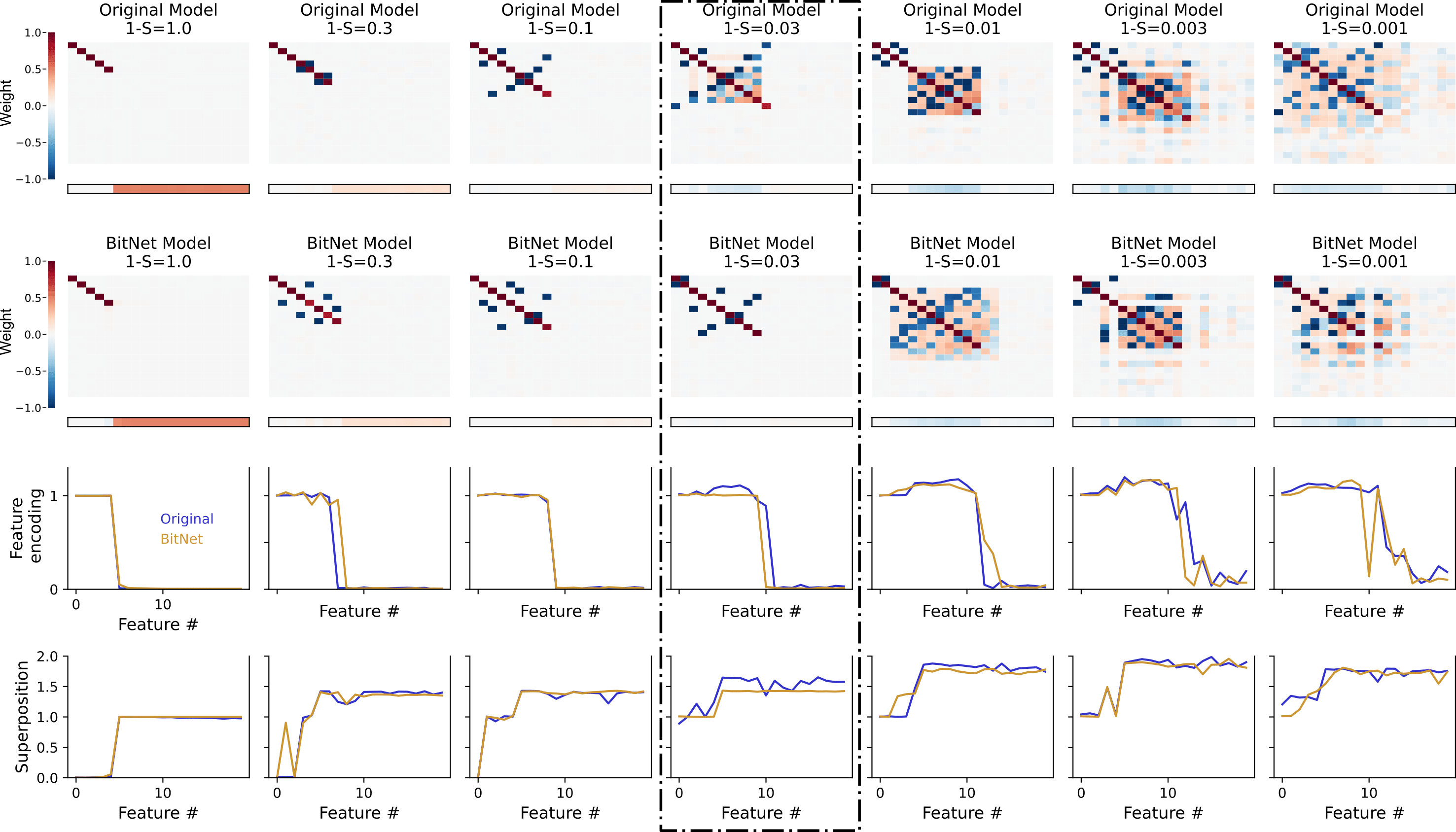
What I plot in the first two rows, mimicking their way of reporting these results, is the $W^{T}W$ matrix - a (features, features) matrix and the vector of biases (b, of length features). If $W^{T}W$ was a diagonal matrix, it would mean that there is a perfect mapping between neurons and features (i.e., monosemantic neurons). In the first row, I reproduce their results; in the second row, I show the equivalent plot for BitLinear. When plotting these two together, although there is a rough match between both network types (in terms of how features are encoded), I noticed three things:

a) when comparing the $W^{T}W$ matrices, there seems to be a later superposition onset for the BitNet case (see how they compare at $1-S=0.03$, highlighted with a dotted rectangle).

b) biases also become negative later on (look at the same sparsity value as before). As they argue:

"the ability to set a negative bias is important for superposition [...] [because] roughly, it allows models to discard small amounts of noise."

c) there is at least one sparsity value ($1-S=0.03$) in which BitNets display less superposition.

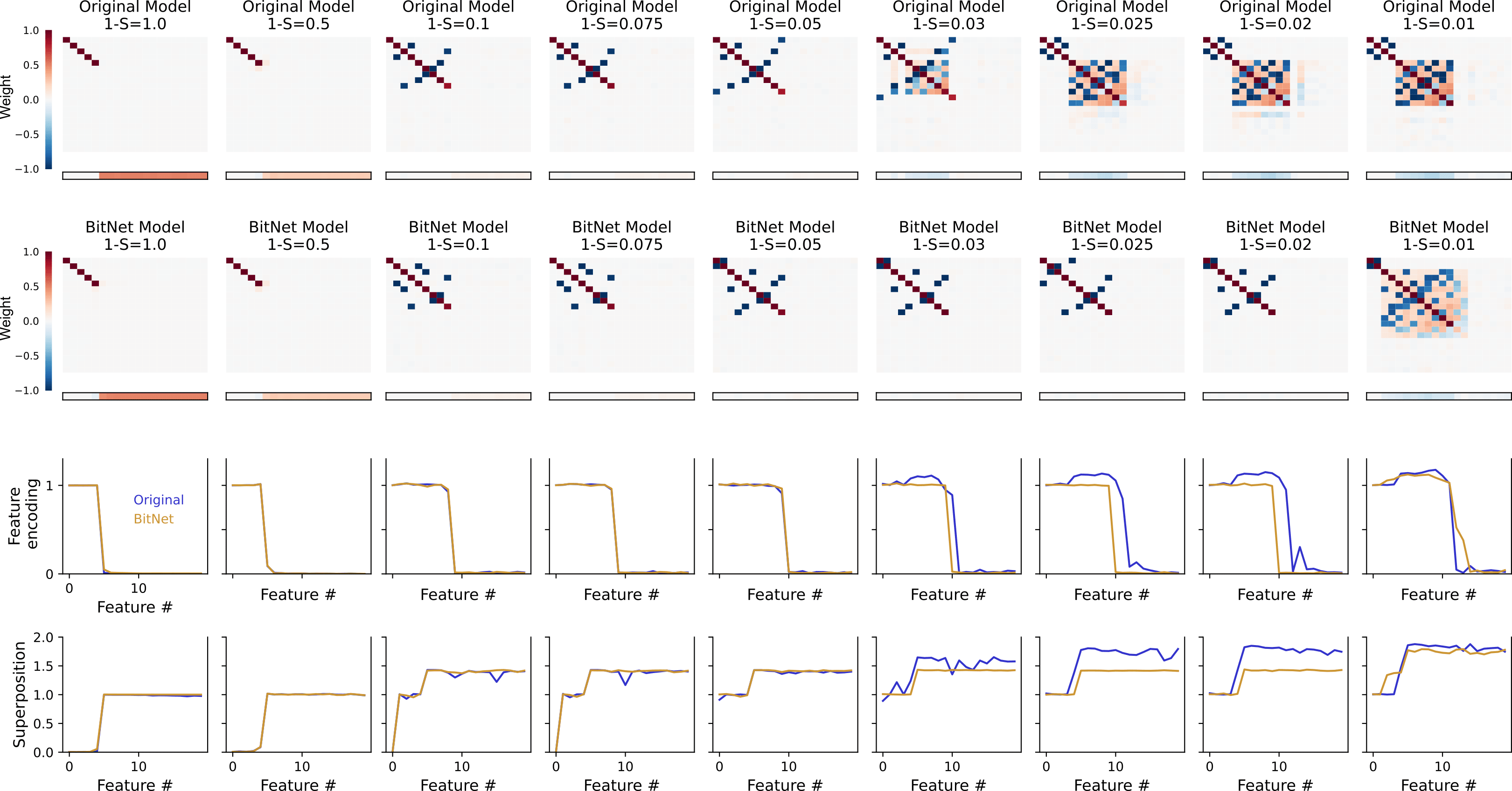
To inspect these observations a bit closer, I zoomed in the sparsity regions in which I thought this difference might happen (around the highlighted region of $1-S=0.03$).

As I guessed, there seems to be a wider sparsity range in which the BitLinear network feature superposition has more structure than the one in regular networks: while the top row has more off diagonal terms of variable strength, the BitLinear one presents only antipodally located features. Accordingly, the bias vector is not negative until larger sparsities (when the antipodal structure is lost). Also, for sparsity values around $1-S=0.03$, the BitNet shows lower superposition (while encoding a similar number of features).

BitLinear networks seem to show a similar geometry of feature superposition

Uniform superposition

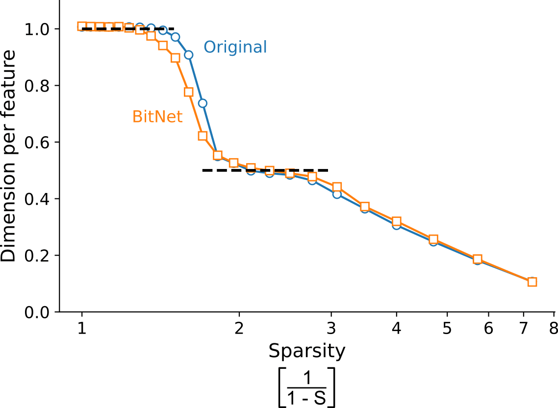
I began by reproducing their results on uniform superposition, where all features are equally important ($I_i=1$). As in their case, I used $n=400$ features and $m=30$ hidden neurons. Similarly to before, a way to measure the number of learned features is by looking at $\left|\right|W|{|}_F^2$, given that $\left|\right|W_i|{|}_F^2\approx 1$ if a feature $i$ is represented and it is $0$ otherwise. They plot the "dimensions per feature", which is quantified by $D^{\ast }=m/\left|\right|W|{|}_F^2$.

When I plot $D^{\ast }$ over different sparsities (x-axis shown as a log scale, measured as $1/(1-s)$), I reproduce their main result for the original network:

Surprisingly, we find that this graph is "sticky" at $1$ and $1/2$ . [...] On inspection, the $1/2$ "sticky point" seems to correspond to a precise geometric arrangement where features come in "antipodal pairs", each being exactly the negative of the other, allowing two features to be packed into each hidden dimension. It appears that antipodal pairs are so effective that the model preferentially uses them over a wide range of the sparsity regime.

I also report that BitNets exhibit a similar behavior, except, perhaps, for a small sparsity range in which its $D^{\ast }$ is consistently below that of the original network.

Non-uniform superposition

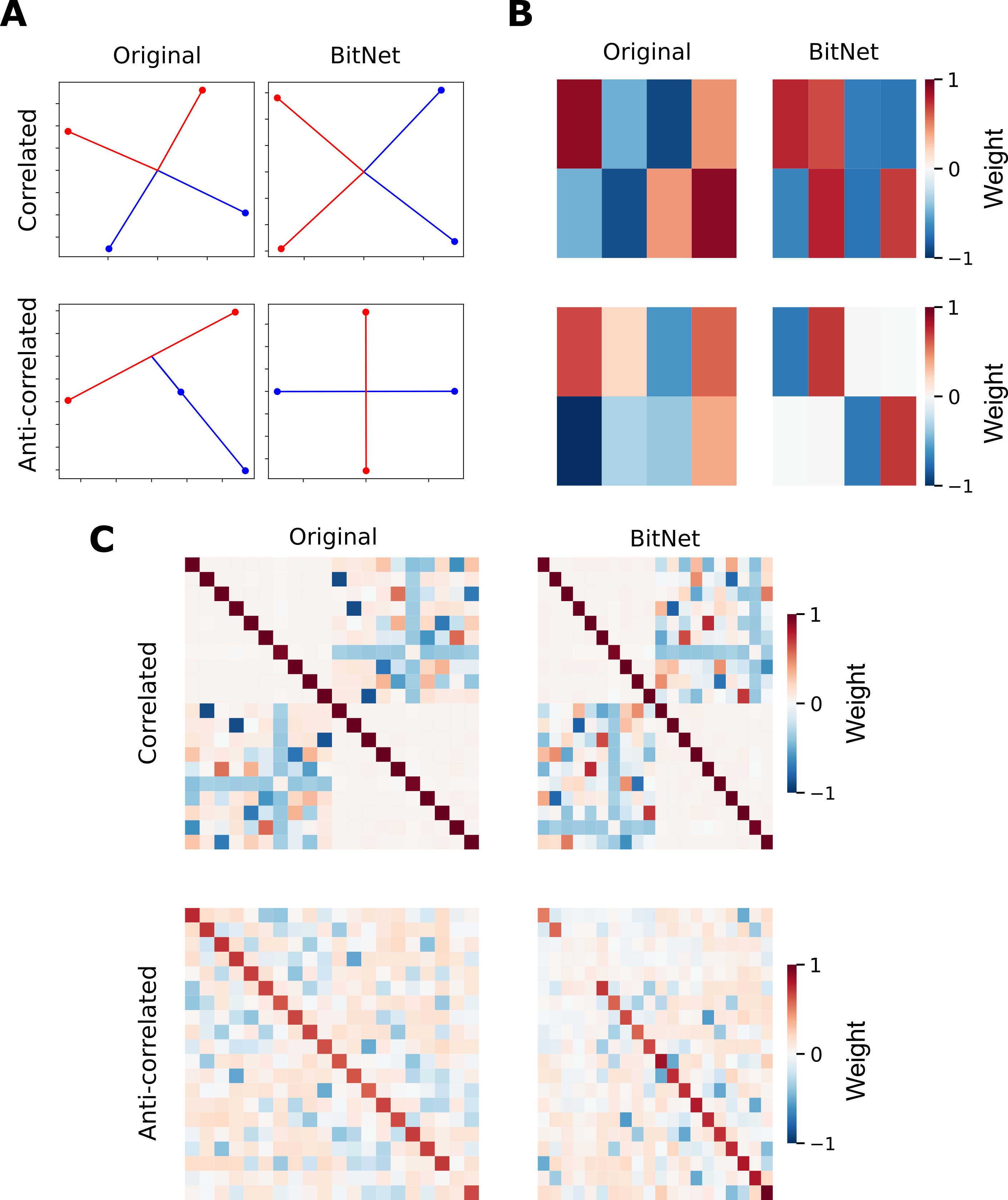
For this part, I followed their implementation of correlated and anti-correlated input features. For the first two panels of this figure, I mirrored their choice of $n=4$ features (correlated by pairs) and $m=2$ hidden dimensions (for easier plotting). For panel C, I moved (as they did) into the case of $n=20$ features (two sets of $10$ correlated ones) and $m=10$ hidden dimensions.

I reproduce their main results:

I) models prefer to represent correlated features in orthogonal dimensions. (See panels A and B).

II) models prefer to represent anticorrelated features in opposite directions. (See panels A and B).

III) models prefer to represent correlated features in orthogonal dimensions, creating "local orthogonal bases". (See panel C, top row).

And I report that these results also hold for the case of BitNets. I think it might be noteworthy that, when inspecting the actual weight matrices (panel B), it is clearer that BitNets encode features more ortogonally than the original networks (which is in line with the previous results that I mentioned in which features are encoded more antipodally in BitNets). For completeness, I also added the case in which features are anti-correlated in two bundles (bottom row).

Conclusion

The take-home message is that BitLinear networks are similar to their dense equivalents in terms of how feature superposition emerges. Perhaps, BitNets have a slight upper hand in some sparsity regimes.

This was a short exploration of how the concepts introduced for the toy models of superposition can be applied to more modern (and efficient) versions of ANNs. As I am currently transitioning into AI Safety, let me know if I have overlooked anything, if any of this is trivial/known already or if I am wrong anywhere! Hopefully this was of interest and it can elicit some interesting discussion!

---

1. Whenever I say "they", unless otherwise stated, I mean the authors from the "Toy Models of Superposition" paper. ↩︎

1 comments

Comments sorted by top scores.