Methodology: Contagious Beliefs

post by James Stephen Brown (james-brown) · 2024-10-19T03:58:17.966Z · LW · GW · 0 comments

Contents

  Simulating Political Alignment
    The Symmetrical Valence Matrix
    Belief Pairs and Valence Values
    Matrix Structure and Calculations
    Simulation Grid
      Agent Representation
      Interaction Rules
      Belief Adoption or Rejection
    Example
      Possible coalitions and their strengths:
      Outcome:
    Why Coalition Strength ≠ Average Valence
      Calculating average valence:
    Why We Don’t Require an Increase in Coalition Strength?
    Correlation
      Calculation Using Phi Coefficient
      Phi Coefficient Formula
    Visualisation and Analysis
      Grid Display
      Correlation Log
    Methodological Considerations
      Symmetry and Limitations
      Addressing Limitations
    Conclusion
None
No comments

Simulating Political Alignment

This methodology concerns a simulation tool which has been developed to model how beliefs, that are not directly related, end up correlated in political identities. It models the transmission of beliefs between nodes on a static hexagonal grid, based on a valence matrix. This methodology allows the user to observe the spread of ideas and the emergence of belief clusters, including correlations between ideas that are not explicitly related.

The model is fully editable but is initially pre-populated with a sample set. This sample set does not reflect objective real-world data.

The Symmetrical Valence Matrix

At the heart of the simulation is the Valence Matrix, where the user can define the relationships between pairs of beliefs. The matrix is symmetrical, meaning that the influence between any two beliefs is the same in both directions. This symmetry simplifies the model and reduces redundancy during data entry—allowing the user to focus on the core interactions without an overwhelming number of parameters.

Belief Pairs and Valence Values

Each belief is represented as a binary pair of opposing extremes (e.g., “Pro-Life” vs. “Pro-Choice”). Valence values range from -100 to +100 and represent the degree of alignment between beliefs:

• Positive Valence (+1 to +100): The presence of one belief increases the likelihood of adopting the other belief.
• Negative Valence (-1 to -100): The presence of one belief decreases the likelihood of adopting the other belief.
• Zero Valence (0): There is no influence between the beliefs.
• Maximum Negative Valence (-100): Represents complete opposition, such as between a belief and its opposing extreme.

Matrix Structure and Calculations

Accounting for the symmetry and binary nature of beliefs, when executed, the code deconstructs the binary pairs into individual belief valences.

• Between a Belief and Its Opposite ($+A$ and $-A$): Always assigned a valence of -100.
• Between Positive Forms of Different Beliefs ($+A$ and $+B$): Valence is defined by the matrix entry  $V$.
• Between Positive and Negative Forms ($+A$ and $-B$): Valence is  $-V$.
• Between Negative Forms of Different Beliefs (-A and -B): Valence is  $+V$.

This can be summarised mathematically:

• $\text{Valence}(+A,+B)=+V$
• $\text{Valence}(+A,-B)=-V$
• $\text{Valence}(-A,+B)=-V$
• $\text{Valence}(-A,-B)=+V$
• $\text{Valence}(+A,-A)=-100$
• $\text{Valence}(+B,-B)=-100$

The value entered in the matrix compares the first (left) side of the binary belief with the first (left) side of the other binary belief. This value is the same when applied to the opposite or values on the right of each binary (due to the symmetrical nature of the model). So, if you have the values {Pro-Tax, Anti-Tax} and the values {Left Wing, Right Wing} with a valence value of 75, this is deconstructed by the program into the following individual valences:

• Pro-Tax vs Left-Wing = +75
• Pro-Tax vs Right Wing = -75
• Anti-Tax vs Left Wing = -75
• Anti-Tax vs Right Wing = +75
• Pro-Tax vs Anti-Tax = -100
• Left Wing vs Right Wing = -100

This approach ensures consistency and reduces the number of unique valence entries needed. For $N$ beliefs, the triangular matrix has $\frac{N(N-1)}{2}$ entries, significantly simplifying the model. For a model with 16 beliefs, this allows for 120 entries (of which many will be left as zero), then each is broken down into 6 individual valences, each representing 2 symmetrical valences. That’s 120 x 6 = 720 valences from the original 120 entries—all of which can have unique correlations when simulated.

Simulation Grid

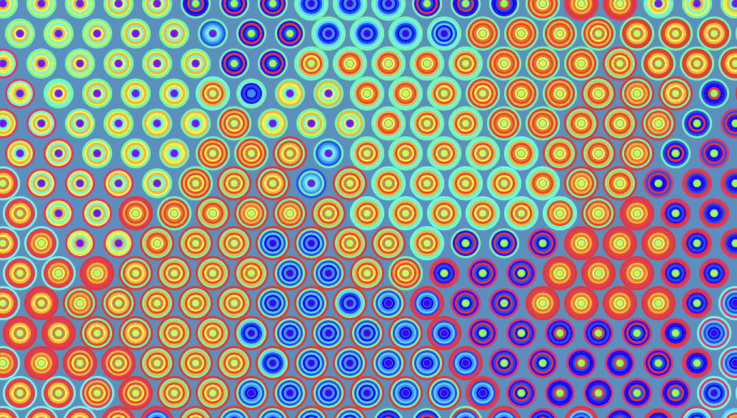
The simulation plays out on a static two-dimensional hexagonal grid, where each node represents an individual agent holding a set of beliefs. The hex grid structure means each agent has exactly six neighbors. Beliefs are randomly seeded to some agents.

Agent Representation

• Beliefs: Each agent possesses a set of beliefs (the agent’s coalition of beliefs).
• Colours: Beliefs are visually represented by coloured rings around each node. Nodes themselves are coloured based on their strongest (most aligned) belief.

Interaction Rules

• Local Influence: Agents interact with their six immediate neighbors. During each simulation step, a random agent transmits a random belief of theirs to their neighbors.
• Valence Application: The influence between agents’ beliefs is calculated using the individual valences derived from the symmetrical valence matrix.

Belief Adoption or Rejection

• An agent’s coalition strength is determined by the sum of all pairwise valences among the beliefs in the coalition.
• An incoming belief is adopted if it does not decrease the agent’s coalition strength.
• If the incoming belief decreases the strength of the coalition (because it conflicts with one or more pre-existing beliefs), then all possible coalitions (subsets) of the current beliefs plus the incoming belief are tested to see which combination has the highest coalition strength.
• Any beliefs not in the strongest coalition are rejected. This may result in the rejection of the incoming belief or the ejection of one or more pre-existing beliefs.

Example

Suppose we have an agent with pre-existing beliefs $A$ and $B$, which share a +10 valence, and an incoming belief $C$ has a +20 valence with A but a -30 valence with $C$:

Possible coalitions and their strengths:

• $(A,B,C)$ = 10 + 20 - 30 = 0
• $(A,B)$ = +10
• $(A,C)$ = +20
• $(B,C)$ = -30

Outcome:

    •    The highest coalition strength is $+20$ for coalition$(A,C)$.
    •    Belief $B$ is ejected, and the agent adopts beliefs $A$ and $C$.

Why Coalition Strength ≠ Average Valence

The reason we use the sum of the valences to determine coalition strength, rather than the sum divided by the number of beliefs (the average valence), is because averaging creates a non-intuitive result. An incoming belief with a positive correlation with both of an agent’s two pre-existing beliefs should always be accepted. But if we are looking at average valence, then the incoming belief needs to have an equal or greater valence than the pre-existing beliefs have with each other.

For example:

    •    Existing Beliefs: Beliefs $A$ and $B$ with  $\text{Valence}(A,B)=+20$.
    •    Incoming Belief: $C$, with  $\text{Valence}(A,C)=+10$  and  $\text{Valence}(B,C)=+10$.

Calculating average valence:

    •    Existing coalition $(A,B):$
    •    Average valence:  $\frac{+20}{1}=+20$
    •    Proposed coalition $(A,B,C):$
    •    Sum of valences:  $+20+(+10)+(+10)=+40$
    •    Number of belief pairs: 3
    •    Average valence:  $\frac{+40}{3}\approx$ +13.33

In this case, the average valence decreases when adding belief $C$, even though all valences are positive. This would incorrectly suggest that belief $C$ should be rejected. Using the sum of valences avoids this issue and aligns with the logic that positive correlations should lead to belief adoption.

Why We Don’t Require an Increase in Coalition Strength?

Similarly, if we require an increase in coalition strength in order to adopt a belief, then an agent with no beliefs will never adopt a belief. The logic of the model is that beliefs are accepted freely until they conflict with existing beliefs.

Correlation

Calculation Using Phi Coefficient

The simulation tracks and logs correlations between beliefs over time. The Phi coefficient is used to measure the correlation between pairs of beliefs.

Phi Coefficient Formula

For binary variables $A$ and $B$:
$\varphi =\frac{P_{AB}-P_A{P}_B}{\sqrt{P_A(1-P_A)P_B(1-P_B)}}$

Where:

• $P_{AB}$: Probability that both beliefs $A$ and $B$ are present in the same agent.
• $P_A$: Probability that belief $A$ is present.
• $P_B$: Probability that belief $B$ is present.

Interpretation

• $\varphi =+1$ : Perfect positive correlation.
• $\varphi =-1$ : Perfect negative correlation.
• $\varphi =0$ : No correlation.

Due to the effects of indirect valences, strong positive or negative correlations can arise between beliefs where there was no assigned valence, or sometimes even in the opposite direction to an assigned valence.

Visualisation and Analysis

Grid Display

• Colour-Coded Agents: The grid visually represents agents’ beliefs. By giving meaningful colours to the beliefs, one can visually track belief propagation and clustering.
• Interactive Inspection: Hovering over an agent reveals a list of that agent’s beliefs.

Correlation Log

• The simulation tracks and logs correlations between beliefs over time, charting them next to the assigned valences between individual beliefs, providing a means for comparison and analysis.

Methodological Considerations

Symmetry and Limitations

1. Symmetrical Relationships: While symmetry simplifies the model, it limits the ability to represent asymmetric influence, where one belief might influence another differently than vice versa.
2. Binary Beliefs: Representing beliefs as binary opposites simplifies the interactions but doesn’t capture nuances such as degrees of belief or non-binary positions.
3. Ignores Social Pressure: While a propensity to increase cognitive coherence and avoid cognitive dissonance is characteristic of belief adoption in human brains, social pressure is also very important and hasn’t been explicitly modelled in this simulation.
4. Doesn't explicitly address Bias: Bias is also a key factor in belief adoption which isn't explicitly addressed in this model.

Addressing Limitations

1. Symmetrical Relationships: Using symmetrical relationships reduced redundancy while testing, where, with respect to political alignment, relationships tended to be symmetrical (requiring duplicate entries of the same values). This symmetry has limitations for applying the model to other areas like health, where a factor like ‘exercise’ might increase ‘tiredness’ (suggesting a positive valence) but ‘tiredness’ might decrease ‘exercise’ (suggesting a negative valence in the other direction). This limitation could be addressed by having a full matrix (rather than a triangular half-matrix) where the top/left triangle of values auto-fills the bottom/right values, but the bottom/right values can be edited manually without affecting the top/left values—balancing efficiency with flexibility. Something to look for in correlations is if there are any consistent asymmetrical correlations that occur despite the symmetrical valences.
2. Binary Beliefs: Representing binary beliefs allows for numerous data points to be added to the simulation from limited entries (6 relationships rather than 1 for each valence value). This does allow for nuance but requires careful application of values and consideration of the actual relationship of one binary belief to another. For a belief like ‘Agnosticism’, which is by definition not on an extreme in the dimension of religious belief, can, however, be paired with ‘Dogmatism’, which is its opposite in the dimension of certainty. This can be a difficult process, and it might be a worthwhile feature to allow for the entry of individual factors that are not binary.
3. Ignores Social Pressure: While the simulation ignores social pressure, the physical nature of the map goes some way to allowing for social pressure in the form of repeated transmission of ideas by neighbours. So that, as soon as a vulnerability in an agent’s belief coalition appears, their neighbours may influence them. I am satisfied with the level at which this simulation aligns with social pressure. To develop a system that enables avoidance might add nuance but would also introduce complications to the model, making result less clear.
4. Doesn't explicitly address Bias: While the model doesn’t explicitly address bias, it is actually founded on the principle of cognitive bias. By having pre-existing beliefs determine the adoption or rejection of incoming beliefs, the rules of the simulation model cognitive bias as a feature of belief adoption rather than a bug (although the more its more buggy attributes are also an emergent property of the model). So, the model doesn't need a separate explicit factoring of cognitive bias.

Conclusion

This simulation offers a framework for exploring how beliefs interact and spread within a population. By utilising a symmetrical valence matrix and a hexagonal grid, we can observe patterns of belief clustering and propagation. While the model abstracts many real-world complexities, it serves as a valuable tool for visualising ideological dynamics and fostering a deeper understanding of belief systems.

Note: This methodology outlines a simplified model designed for exploratory purposes. Real-world belief dynamics involve asymmetries, degrees of belief, and complex network structures not fully captured in this simulation. While the valence matrix is pre-populated with example values, these values are based on the author's intuitive understanding, and are not strictly data-driven—these are intended to be edited by the user to test their own parameters.

0 comments

Comments sorted by top scores.