SGD Understood through Probability Current

post by J Bostock (Jemist) · 2021-12-19T23:26:23.455Z · LW · GW · 1 comments

Contents

  Gradient Variance
  Validation of the First Term of the Equations
  Validation of the Second Term of the Equations
  Solving for End-States
  What's the point?
  Further Investigation
None
1 comment

My previous post about SGD was an intro to this model. That post concerned a model of a loss landscape on two "datapoints". In this post I attempt to build a new model of SGD and validate it, with mixed success, but it is sort of interesting.

Gradient Variance

We could model this another way. The expected change of $W$ on each step is $-T\frac{dW}{dL}$, but we will also expect variance. $W$ will evolve over time through probability space. There are two competing "forces" here, the "spreading force" created by variance in in $\frac{dW}{d{l}_j}$ over all datapoints in the model, and the "descent force" being exerted by gradient descent pushing $W$ back into the centre of a given local minimum.

I think it makes sense to introduce some new notation here.

$g_j\left(W\right)=\frac{d{l}_j}{dW}$ 

$G\left(W\right)=\frac{dL}{dW}=averag{e}_{\left(allj\right)}\left(g_j\right(W\left)\right)$

$S^2\left(W\right)=varianc{e}_{\left(allj\right)}\left(g_j\right(W\left)\right)$ 

$S\left(W\right)=+\sqrt{S^2\left(W\right)}$

The $S^2$ notation should be thought of like the $co{s}^2\left(x\right)$ notation.

Plotting these for our current system:

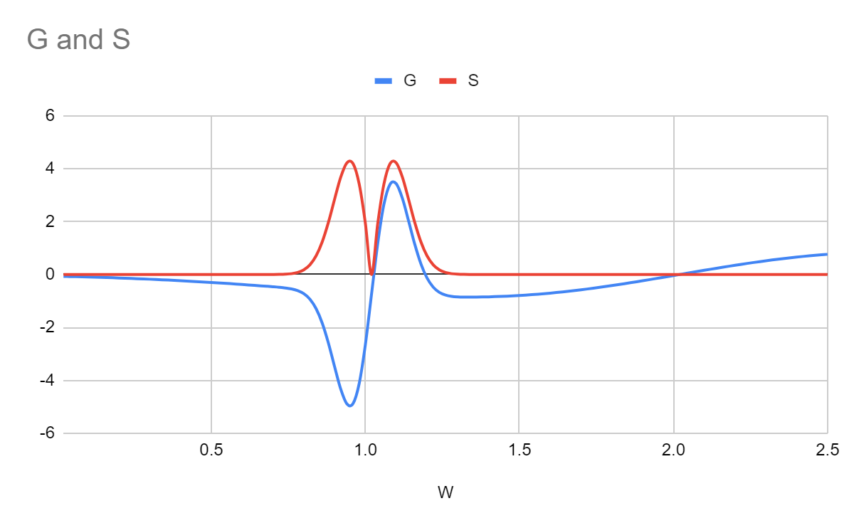
Places where $G$ is zero and the gradient of $G$ is positive are the stable equilibrium points with regards to gradient descent on $L$ (at ~1 and 2). If $G$ and $S^2$ are both zero at the same place, then this is an equilibrium point with regards to SGD on $L$ (only at 2). The zero points for $G$ and $S^2$ around the pit at 1 are not quite in the same pace.

It is possible to consider probability mass of $W$ "moving" according to the following rule:

A "point" (dirac $\delta$ distribution) of probability at $W$, between $t$ and $t+1$, changes to a distribution centred at $W-TG\left(W\right)$ with a variance of $T^2{S}^2\left(W\right)$. 

Now we have abstracted away $T$ from the actual process of discontinuous updates, we can try and factor out the discontinuity entirely. This will make the maths more manageable when it comes to generalizing to larger models. $T$ will likely be much smaller for larger models but as long as $S\left(W\right)$ grows larger with the number of datapoints used, this will compensate.

(Point of notation, I will be using $d$ rather than $\partial$, even though the latter is arguably more correct. As we will never be "mixing" $W$and $t$ it won't make a difference to our results)

Instead of probability distribution moving, we might now consider it flowing. This can be described by a probability current density $\rho$:

Consider a system with $S^2\left(W\right)=0$ everywhere. The probability will just flow down the gradient:

$\rho (W,t{)}_G=-TG(W\left)P\right(W,t)$

Taking $\frac{dP}{dt}=-\frac{d\rho }{dW}$ we get (when dependencies are removed for ease of reading):

${\frac{dP}{dt}}_G=T[G\frac{dP}{dW}+P\frac{dG}{dW}]$

Now consider a system with $G\left(W\right)=0$ everywhere. Now we effectively have the evolution of a probability distribution via random walk. This gives a "spreading out" effect. With constant $S^2$ we have the following equation for $\rho$, borrowed from the heat equation. I will take the central limit theorem and assume that the gradients are normally distributed.

$\rho (W,t{)}_S=-\frac{1}{2}{T}^2{S}^2\frac{dP(W,t)}{dW}$

Based on the fundamental solution of the heat equation this will increase our variance by $T^2{S}^2$ each step of $t$.

Which gives us:

${\frac{dP}{dW}}_S=\frac{1}{2}{T}^2{S}^2\frac{d^{2}P}{dW}+\frac{1}{2}{T}^2\frac{d\left(S^2\right)}{d{W}^2}\frac{dP}{dW}$

But the speed of "spreading out" is proportional to $S\left(W\right)$ which changes the equation. The slower the "spreading out", the higher the probability of $W$ being there. This makes $S\left(W\right)$ act like a "heat capacity" of the location for $P(W,t)$ for which $\rho$ is a conserved current. We might be able to borrow more from heat equations. In this case $P(W,t)S\left(W\right)$ acts as the "temperature" of a region.

$\rho (W,t{)}_S=-k(W)\frac{d\left[P\right(W,t\left)S\right(W\left)\right]}{dW}$

$\rho (W,t{)}_S=-k(W\left)\right[S\left(W\right)\frac{dP(W,t)}{dW}+P(W,t)\frac{dS\left(W\right)}{dW}]$

Calculating $k$ based on our previous equation gives $k\left(W\right)=\frac{1}{2}{T}^{2}S\left(W\right)$, which gives:

${\frac{d\rho }{dW}}_S=-\frac{d}{dW}[-\frac{1}{2}{T}^2{S}^2(W)\frac{dP(W,t)}{dW}-\frac{1}{2}{T}^{2}S(W\left)P\right(W,t\left)\frac{dS\left(W\right)}{dW}\right]$

This can be reduced to the rather unwieldy equation (removing function dependencies for clarity):

${\frac{dP}{dt}}_S=T^2[\frac{3}{2}S\frac{dS}{dW}\frac{dP}{dW}+\frac{1}{2}{S}^2\frac{d^{2}P}{d{W}^2}+\frac{1}{2}(\frac{dS}{dW}{)}^{2}P+\frac{1}{2}SP\frac{d^{2}S}{d{W}^2}]$

But these can be expressed in terms of $S^2$ rather than $S$, which is good when $S$ is pathological in some way (like when $S^2$ is zero above, $S$ has a discontinuous derivative). It also makes sense that our equation shouldn't depend on our choosing positive rather than negative $S$.

${\rho }_S=-T^2[\frac{1}{2}{S}^2\frac{dP}{dW}+\frac{1}{4}P\frac{d\left(S^2\right)}{dW}]$

${\frac{dP}{dT}}_S=T^2[\frac{3}{4}\frac{d\left(S^2\right)}{dW}\frac{dP}{dW}+\frac{1}{2}{S}^2\frac{d{P}^2}{dW}+\frac{1}{4}\frac{d^2\left(S^2\right)}{d{W}^2}P]$

Finally giving our master equations:

$\rho =-T^2[\frac{1}{2}{S}^2\frac{dP}{dW}+\frac{1}{4}\frac{d\left(S^2\right)}{dW}P]-T\left[GP\right]$

$\frac{dP}{dt}=T^2[\frac{3}{4}\frac{d\left(S^2\right)}{dW}\frac{dP}{dW}+\frac{1}{2}{S}^2\frac{d{P}^2}{dW}+\frac{1}{4}\frac{d^2\left(S^2\right)}{d{W}^2}P]+T[G\frac{dP}{dW}+P\frac{dG}{dW}]$

Validation of the First Term of the Equations

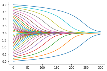
Let's start with the first equation, and simulate using our G function from before.

T = 0.02, no stochasticity yet.

Here's $W$ on the y-axis, and $t$ on the x-axis. This is what the evolution of $W$ looks like for a series of initial $W$ values:

Now let's pick a couple of initial distributions and see how they evolve over time:

Time evolution with steps of $\Delta t=10$:

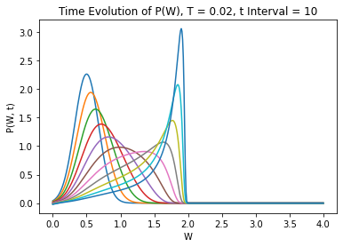
This looks about right!

Now let's plot the mean of this over time, and compare to the mean and standard deviation of a Monte Carlo simulation of gradient descent. The Monte Carlo simulation starts with 1000 $W$ values chosen to form a normal distribution with the roughly same mean and standard deviation (0.5 and 0.175 respectively) as our initial $P(W,t)$ distribution.

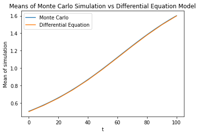
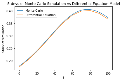
Our first equation is an accurate description of non-stochastic gradient descent. The rest of the difference in the standard deviation is most likely due to imperfect matching of our initial data ($P$ is a truncated normal distribution but our Monte Carlo uses a normal distribution with matched mean and variance to the truncated $P$, so some elements are $<0$ where the gradient is small).

Validation of the Second Term of the Equations

Let's take our first example as a distribution spreading out. 

$g_0=-1,g_1=1,G=0,S^2=1$

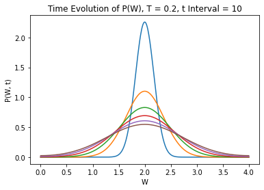
And compare standard deviations to our Monte Carlo simulation:

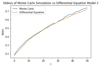
Looking good, errors here may also be due to truncation.

One final validation step: take $g_0=1.2W-2$,  $g_1=0.8W-2$, $G=W-2$, $S^2=0.4W^2$, $T=0.5$. This model will be used to assess a few things: our ability to perform well at higher $T$, its ability to predict the correct form of the counterbalancing "concentrating" and "spreading" forces of $G$ and $S^2$, and its ability to predict the concentration of probability mass in regions of lower $S^2$.

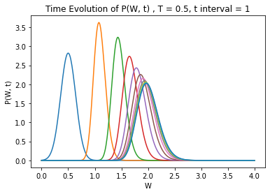
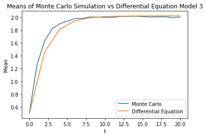
Unfortunately the computational modelling seems to fall apart when applied to the original system. The large first and second derivatives of $S^2$ lead to a lot of instability. This means I can't validate it much more than this. High values of $T$ also cause the model to break down, as the gradient might change a lot in the span of a step. I think this can be remedied by (for example) picking a $g$ to update on and updating with multiple small steps before changing $g$.

I'm no master programmer and I don't have much experience working with unstable PDEs. So I can't do much more here.

Solving for End-States

For an end-state, $\rho =0$ everywhere. This means:

$0=-T^2[\frac{1}{2}{S}^2\frac{dP}{dW}+\frac{1}{4}\frac{d\left(S^2\right)}{dW}P]-T\left[GP\right]$

$T\frac{1}{2}{S}^2\frac{dP}{dW}=-T\frac{1}{4}\frac{d\left(S^2\right)}{dW}P-GP$

$\frac{dP}{dW}\frac{1}{P}=-\frac{1}{2S^2}\frac{d\left(S^2\right)}{dW}-\frac{2G}{T{S}^2}$

$\frac{d\left(log\right(P\left)\right)}{dW}=-\frac{1}{2S^2}\frac{d\left(S^2\right)}{dW}-\frac{2G}{T{S}^2}$

$\frac{d\left(log\right(P\left)\right)}{dW}=-\frac{1}{2}\frac{d\left(log\right(S^2\left)\right)}{dW}-\frac{2G}{T{S}^2}$

This shows our problem. When $S^2$ vanishes, our equations don't work terribly well. We might have to hope that the two opposing $S^2$ terms cancel out and it works, but who knows. This is probably the source of instability in our equations.

But around some minimum it lets us interpret something. If $log\left(P\right)$ is decreasing linearly then $P$ decreases exponentially. Let's consider the $\frac{2G}{T{S}^2}$ term now. If we have two minima (with a maximum between them) around which the loss landscapes are exactly the same, except one is twice as wide (in all $l_i$) then the $G$ component will be halved in the wider one, but the $S^2$ part will be quartered. This means the integral of $\int -\frac{2G}{T{S}^2}dW$ from the centre of the wider one to the maximum will be four times that of the narrower one. Therefore the probability density at the centre of the wider minimum's basin will be e^4 = 56 times Edit: a lot higher.

What's the point?

Reasoning about stochastic processes is difficult. Reasoning about differential equations is also difficult, but the tools to analyse differential equations are different and might be able to solve different problems.

SGD is believed to have certain "bias" towards low-entropy models of the world. Part of this is a preference for "broader" rather than "narrower" minima in $L$. Now we have some tools which may allow us to understand this. Under this model, SGD is also biased towards regions of low variance in loss function.

Further Investigation

I think there's something like a metric acting on a space here. $S^2$ looks like a metric, and perhaps it's actually more correct to consider the space of $W$ with the metric such that $S^2=1$ everywhere. For higher dimensions we get the following transformations:

$W\to \overrightarrow{W}$
$G\to \overrightarrow{G}$
$S^2\to S^2$

Now $\overrightarrow{W}$ and $\overrightarrow{G}$ are vectors and $S^2$ is a matrix. This extends nicely as we can choose our metric such that $S^2=I$. It might be useful to define some sort of function like an "energy" over the landscape of \(\\)$W$ in terms of $G$, $S$, and $T$ alone which describes the final probability distribution. In fact such a function must exist assuming SGD converges, as $log\left(P\right(W,\infty \left)\right)$ is well-defined. What the actual form of this function is would require to do some working out, and it may not be at all easily described. This whole process is very reminiscent of both chemical dynamical modelling and finding the minimum-energy configuration of a quantum energy landscape, as both consist of a "spreading" term and an "energy" term.

While it is quite interesting, I don't consider this a research priority for myself. About 90% of this post has been sitting in my drafts for the past 3 months. Even if powerful AI is created using SGD, I'm not convinced that this sort of model will be hugely useful. It might be possible to wrangle some selection-theorem-ish-thing out of this but I don't think I'll focus on it.

1 comments

Comments sorted by top scores.