Climate technology primer (1/3): basics
post by amarbles · 2019-10-25T23:18:09.351Z · LW · GW · 5 commentsContents
  Basic numbers on climate
    Radiation balance
    Climate sensitivity
      Water vapor
      Ocean biology effects
      Land biology effects
      Permafrost
      Local warming
      The need for detailed and complex simulations
      Let’s try to ballpark the feedback effects anyway!
        Without any feedback:
        With a historical estimate of feedback:
      Potential tipping points
      A middle of the road climate sensitivity
      Implications of the middle of the road climate sensitivity for carbon budgets
    Impacts
      Some baseline scenarios for sea level rise
      Implications of potential tipping points in ice melt
    Emissions
      Sectors driving emissions
      Evaluating some popular ideas about emissions reduction
      A bit about clean electricity, renewables, storage, nuclear, and the power grid
      How quickly must we fully decarbonize?
      The need for a (revenue-neutral, staged) carbon tax
      Tentative conclusions
None
5 comments
This is my first post here, cross-posted from
https://longitudinal.blog/co2-series-part-1-review-of-basics/
Posting was suggested by Vaniver, and the actual work of cross-posting was done by Benito.
Comments appreciated. (Will only cross post the first of the 3 climate posts here.)
This is the first of a series of three blog posts intended as a primer on how technology can help to address climate change.
Note: you can annotate this page in Hypothes.is here: https://via.hypothes.is/https://longitudinal.blog/co2-series-part-1-review-of-basics/
Excellent documents and courses are available online on what we are doing to the climate — such as the IPCC reports or Prof. Michael Mann’s online course or this National Academies report. Even more so, this type of open source analysis is what the field needs to look like. But I had to dig a bit to see even the beginnings of a quantitative picture of how technologies can contribute to solving the problems.
There are integrative assessments of solutions, such as Project Drawdown, and a huge proliferation of innovative technologies being proposed and developed in all sectors. There are also some superb review papers that treat the need for new technologies. Bret Victor has a beautiful overview emphasizing the role of general design, modeling and implementation capacity, and there is now a climate change for computer scientists course at MIT. But, as a scientifically literate (PhD in Biophysics) outsider to the climate and energy fields, I was looking to first understand the very basics:
- How can I estimate the world’s remaining carbon budget for various levels of warming? What are the uncertainties in this?
- What would happen if Greenland melted?
- What are the fundamental physical limits on, say, the potential for sucking carbon dioxide out of the atmosphere? How low could the cost theoretically go?
- How many trees would you need to plant, and are you going to run out of water, land or fertilizer for them?
- If we did manage to remove a given amount of CO2, how would the climate respond? How would the climate respond if we magically ceased all emissions today?
- What would be the real impact if we could electrify all cars?
- Are batteries going to be able to store all the variable renewable energy we’ll need? Is there enough Uranium obtainable to power the world with nuclear? Order of magnitude, how much would it cost to just replace our entire energy supply with nuclear?
- Notwithstanding the complexity of their governance and potential moral hazard implications, do we have a solid science and engineering basis to believe that any geoengineering methods could theoretically work to controllably lower temperature, and if so, would that be able to slow down sea ice melt, too? Would it damage the ozone layer? How fast could you turn it off? Could it be done locally?
- Etc.
For questions like those and many others, I want to calculate “on the back on an envelope” an estimate of whether any given idea is definitely crazy, or might just be possible.
I suspect that a similar desire led the information theory and statistics luminary David MacKay to write his seminal calculation-rich book Sustainable Energy without the Hot Air. While these blog posts, written over a few vacations and weekends by a more modest intellect, don’t begin to approach MacKay’s standard of excellence, I do hope that they can serve as a breadcrumb trail through the literature that may help others to apply this spirit to a broader set of climate-relevant engineering problems.
In this first of three posts, I attempt an outsider’s summary of the basic physics/chemistry/biology of the climate system, focused on back of the envelope calculations where possible. At the end, I comment a bit about technological approaches for emissions reductions. Future posts will include a review of the science behind negative emissions technologies, as well as the science (with plenty of caveats, don’t worry) behind more controversial potential solar radiation management approaches. This first post should be very basic for anyone “in the know” about energy, but I wanted to cover the basics before jumping into carbon sequestration technologies.
(These posts as a whole are admittedly weighted more towards what I perceived to be less-mainstream topics, like carbon capture and geo-engineering. In this first one, while I do briefly cover a lot of cool mitigation techniques — like next-generation renewables storage, a bit about nuclear, and even a bit about the economics of carbon taxes — I don’t try to cover the full spectrum of important technology areas in mitigation and adaptation. But don’t let that leave you with the impression that the principal applications of tech to climate are in CO2 removal and geo-engineering. Areas I don’t cover much here may be even more important and disruptive — like, to name a few, decarbonizing steel and cement production, or novel control systems for solar and wind power, or the use of buildings as smart grid-adaptive power loads, or hydrogen fuel, or improved weather prediction… It just happens that the scope of my particular review here is: some traditional mitigation, a lot of CDR and geo-engineering, and ~nothing in adaptation aspects like public health or disaster relief. Within applications of machine learning to climate, I recommend this paper for a broader picture that spans a wider range of solution domains — such breadth serves as good food for thought for technologists interested in finding the truly most impactful areas in which they might be able to contribute, but I don’t attempt it here.)
Disclaimers:
- I am not a climate scientist or an energy professional. I am just a scientifically literate lay-person on the internet, reading up in my free time. If you are looking for some climate scientists online, I recommend those that Michael Nielsen follows, and this list from Prof. Katharine Hayhoe. Here are some who apparently advise Greta. You should definitely read the IPCC reports, as well, and take courses by real climate scientists, like this one. The National Academies and various other agencies also often have reports that can claim a much higher degree of expertise and vetting than this one.
- Any views expressed here are mine only and do not reflect any current or former employer. Any errors are also my own. This has not been peer-reviewed in any meaningful sense. If you’re an expert on one of these areas I’ll certainly appreciate and try to incorporate your suggestions or corrections.
- There is not really anything new here — I try to closely follow and review the published literature and the scientific consensus, so at most my breadcrumb trail may serve to make you more aware of what scientists have already told the world in the form of publications.
- I’m focused here on trying to understand the narrowly technical aspects, not on the political aspects, despite those being crucial. This is meant to be a review of the technical literature, not a political statement. I worried that writing a blog purely on the topic of technological intervention in the climate, without attempting or claiming to do justice to the social issues raised, would implicitly suggest that I advocate a narrowly technocratic or unilateral approach, which is not my intention. By focusing on technology, I don’t mean to detract from the importance of the social and policy aspects. I do mention the importance of carbon taxes several times, as possibly necessary to drive the development and adoption of technology. I don’t mean to imply through my emphasis that all solutions are technologically advanced — for example, crucial work is happening on conservation of land and biodiversity. That said, I do view advanced technology as a key lever to allow solutions to scale worldwide, at the hundreds-of-gigatonnes-of-CO2 level of impact, in a cost-effective, environmentally and societally benign way. Indeed, the rights kinds of improvements to our energy system are likely one of the best ways to spur economic growth.
- Talking about emerging and future technologies doesn’t mean we shouldn’t be deploying existing decarbonization technologies now. There is a finite cumulative carbon budget to avoid unacceptable levels of warming. A perfect technology that arrives in 2050 doesn’t solve the primary problem.
- For some of the specific technologies discussed, I will give further caveats and arguments in favor of caution in considering deployment.
Acknowledgements: I got a bunch of good suggestions from friends including Brad Zamft, Sarah Sclarsic, Will Regan, David Pfau, David Brown, David Rolnick, Tom Hunt, Tony Pan, Marcus Sarofim, Michael Nielsen, Sam Rodriques, James Ough, Evan Miyazono, Nick Barry, Kevin Esvelt, Eric Drexler and George Church.
Outline:
- Introduction
- Basic numbers on climate
- Radiation balance
- Climate sensitivity
- Water vapor
- Ocean biology effects
- Land biology effects
- Permafrost
- Local warming
- The need for detailed simulations
- Trying to ballpark the feedbacks
- Without feedback
- With historical factor of 4
- Potential tipping points
- With 450 ppm ~ 2C middle of the road estimate
- Implications of middle of the road estimate
- Impacts
- Baseline scenarios for sea level rise
- Potential tipping point scenarios for ice melt
- Emissions
- Sectors
- Evaluating some popular ideas: electric cars and less air travel
- A bit about clean electricity, nuclear and the power grid
- How quickly must we decarbonize?
- Carbon tax
- Tentative conclusions
Basic numbers on climate
Let’s start with crude “back of the envelope” approximations — of a type first done by Svante Arrhenius in 1896, who got the modern numbers basically right — and see how far we get towards understanding global warming (the phenomenon of CO2-driven warming itself was arguably discovered around 1856 by Eunice Foote). We’ll quickly hit a complexity barrier to this approach, but the lead-up was interesting to me.
Radiation balance
The atmosphere is complicated, many layered, and heterogeneous. But as a quick tool for thought, we can start with simple single-layer atmosphere models, aiming to understand the very basics of the effect of the atmosphere on the Earth’s balance of incoming sunlight versus outgoing thermal infrared radiation. These basics are covered at the following excellent sites
- acs.org/content/acs/en/climatescience/atmosphericwarming/singlelayermodel.html
- web.gps.caltech.edu/classes/ese148a/ especially lecture 2
- mathaware.org/mam/09/essays/Radiative_balance.pdf
- clivebest.com/blog/?p=2241
- assets.press.princeton.edu/chapters/s9636.pdf
- https://geosci.uchicago.edu/~rtp1/papers/PhysTodayRT2011.pdf
- https://en.m.wikipedia.org/wiki/Idealized_greenhouse_model
- https://twitter.com/michael_nielsen/status/1096990267259809793
- https://www.e-education.psu.edu/meteo469/node/198
which I now summarize.
An ideal black body radiator (e.g., a very idealized Planet Earth), with no greenhouse effect, would radiate an energy flux:

where

is the Stefan-Boltzmann constant, and T is the temperature in Kelvin.
If we multiply this flux by the surface area of the Earth, we have the outgoing emitted energy:

If the planet was in radiative balance — so that the incoming solar energy is equal to the outgoing thermal energy and the planet would be neither warming nor cooling — we’d want to set this equal to the incoming solar energy

This last equation introduced the albedo A, which is the fraction of incoming solar energy reflected directly back without being absorbed, and the incoming solar flux S from the sun.
The incoming solar radiation is roughly S = 1.361 kilowatts per square meter, and the albedo A is around 0.3. S is easy to calculate: the sun has a radius of 700 million meters and a temperature of 5,778K, so the energy radiated by the sun is, by the same formula we used for the Earth,

which is then by the time it reaches the Earth spread over a sphere of radius given by the Sun-Earth distance of 1.5e11 meters, so the solar flux per unit area is

(That’s a lot of solar flux. If the area of Texas was covered by 4% efficient solar collection, that would offset the entire world’s average energy consumption.)
We can then solve our incoming-outgoing solar energy balance for the single unknown, the equilibrium temperature T, which comes out to 255 Kelvin or so. Now this is quite cold, below zero degrees Fahrenheit, whereas the actual global mean surface temperature is much warmer that, on average around 60 degrees Fahrenheit (288K or so) — the reason for this difference is the greenhouse effect.
The greenhouse-gas-warmed situation that we find ourselves in is also simple to model at a crude level, but complex to model at a more accurate level.
At the crudest level (first few lectures of an undergraduate climate science course), if a certain fraction ε of outgoing infrared radiation is absorbed by the atmosphere on the way out (e.g., by its energy being converted into intra-molecular vibrations and rotations in the CO2 molecules in the atmosphere), and then re-emitted, then we can calculate the resulting ground temperature (a more complete explanation is in the lead-up to equation 1.15 here, or here), arriving at a ground temperature

where f is the fraction of incoming solar radiation absorbed by the atmosphere before making it to the surface, and ε is the so-called atmospheric emissivity — ε this is zero for no greenhouse gasses and 1 for complete absorption of infrared radiation from the surface by the atmosphere. I’ve seen f = 0.08 (the atmosphere absorbs very little, less than 10%, of the incoming solar radiation), and ε=0.89 although various other combinations do the same job. If you plug this all in, you get a ground temperature of 286 Kelvin or so, which is pretty close to our actual global mean surface temperature of around 288 Kelvin. (Note that even if ε=1, we don’t have infinite warming, as the radiation is eventually re-radiated out to space.)
Here is the picture that goes with this derivation:

Again, this is not a good model, because it neglects almost all the complexities of the atmosphere and climate system, but it can be used to illustrate certain basic things. For example, if you want to keep the Earth’s temperature low, you can theoretically increase the albedo, A, to reflect a higher percentage of the incoming solar radiation back to space; this is called solar geoengineering or solar radiation management, and this formula allows to calculate crudely the kind of impact that can have.
But the formula is hopelessly oversimplified for most purposes, e.g., we’ve neglected the fact that much of the heat leaving the Earth’s surface is actually due to evaporation, rather than direct radiation.
A significantly better framework, yet still fully analytical rather than simulation-based, is provided by this paper (and slides and these three videos), but the physics is more involved.
Climate sensitivity
A key further problem for us as back-of-the-envelope-ers, though, is to know what a given amount of CO2 in the atmosphere translates to in terms of effective ε and A (and f) in the above formula. Or in plain English, to relate the amount of atmospheric CO2 to the amount of warming. This is where things get trickier. Before trying to pin down a number for this “climate sensitivity”, let’s first review why doing so is a very complex and multi-factorial problem.
Water vapor
Naively, if we think of the only effect of CO2 as being the absorption of some of the outgoing infrared thermal radiation from the planet surface, then more CO2 means higher ε, with no change in albedo A. However, in reality, more warming also leads to more water vapor in the atmosphere, which — since water vapor is itself a greenhouse gas — can lead to more greenhouse effect and hence more warming, causing a positive feedback. On the other hand, if the extra water vapor forms clouds, that can increase the albedo, decreasing warming by blocking some of the incoming solar radiation from hitting the surface, and leading to a negative feedback. So it doesn’t seem obvious even what functional form the impact of CO2 concentration on ε and A should take, particularly since water vapor can play multiple roles in the translation process.
If you just consider clouds per se, it looks like they on average cool the Earth, from an experiment described in lecture 10a of the Caltech intro course, but this depends heavily on their geographic distribution and properties, not to mention their dynamics like heating-induced evaporation, changes in large-scale weather systems, effects specific to the poles, and so on. Aerosol-cloud interactions, and their effects on albedo and radiative forcing, appear to be a notable area of limited scientific understanding, and the IPCC reports state this directly. Also, a particular type of cloud called Cirrus actually warms the Earth.
In general, the feedback effects of water are a key consideration and still imperfectly understood by the field, although the research is making great strides as we speak. For example, just looking at a fairly random sampling of recent papers, it looks like the nature of the water feedback may be such that the Stefan-Boltzmann law calculation above is no longer really appropriate even as an approximation, leading to a linear amount of outgoing radiation with temperature rather than quartic per the Stefan-Boltzmann law
phys.org/news/2018-09-earth-space.html
Even weirder,
news.mit.edu/2014/global-warming-increased-solar-radiation-1110
the roles of carbon dioxide and water may be such that the largest warming mechanism is increased penetrance of solar radiation rather than decreased escape of infrared per se. As the article explains:
“In computer modeling of Earth’s climate under elevating CO2 concentrations, the greenhouse gas effect does indeed lead to global warming. Yet something puzzling happens: While one would expect the longwave radiation that escapes into space to decline with increasing CO2, the amount actually begins to rise. At the same time, the atmosphere absorbs more and more incoming solar radiation; it’s this enhanced shortwave absorption that ultimately sustains global warming.”
Note that this paper is meant as an explanation of known phenomena arising inside climate models, not as a contradiction of those models.
So it is complicated. (I don’t mean to over-emphasize these particular papers except to say that people are still discovering core aspects of how the Earth’s energy balance works.)
Moreover, the feedback effects due to changes associated with water take a long time to manifest, due in part to the large specific heat of water and the large overall heat capacity of the enormous, deep oceans, and in part due to the long residence time of CO2 in the atmosphere. Thus, simply fitting curves for observed temperature versus CO2 concentration on a short timescale around the present time may fail to reflect long-timescale processes that will be kicking in over the coming decades, such as feedbacks.
Ocean biology effects
There are also large ocean biology and chemistry effects. Just to list a few, dissolved carbon impacts the acidity of the ocean, which in turn impacts its ability to uptake more carbon from the atmosphere. There are also major ocean biological effects from photosynthesis and the drivers of it. As the Caltech course explains:
“On longer time scales (decade to century), atmospheric CO2 is strongly influenced by mixing of deep ocean water to the surface. Although deep water is generally supersaturated with respect to even the modern atmosphere, mixing of these water masses to the surface tends to draw down atmospheric CO2 in the end as the high nutrients stimulate formation of organic carbon. Several coupled atmosphere-ocean models have shown, however, that global warming is accompanied by an increase in vertical stratification within the ocean and therefore reduced vertical mixing. On its own, this effect would tend to reduce the ocean CO2 uptake. However, changes in stratification may also drive changes in the natural carbon cycle. The magnitude and even the sign of changes in the natural cycle are much more difficult to predict because of the complexity of ocean biological processes…”. Indeed, the Caltech slides invoke localized mixing effects in parts of the ocean, and their impact on ocean photosynthesis, as a possible explanation for major pre-industrial temperature changes on inter-glacial timescales.
Land biology effects
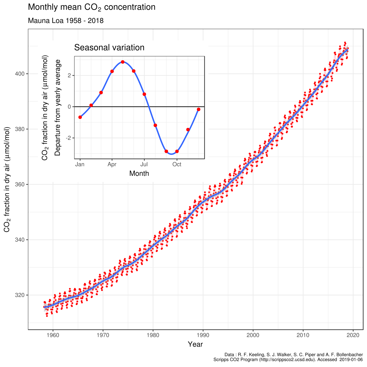
There are also terrestrial biological effects. We’ll use the great physicist Freeman Dyson’s emphasis on these as a jumping off point to discuss them. (Dyson is known as a bit of a “heretic” on climate and many other topics. Here are 157 interviews with him. We won’t dwell on his opinions about what’s good for the world, just on the technical questions he asked about the biosphere, because the history is cool.) In 1977, in a paper that will come up again for us in the context of carbon sequestration technologies, Dyson pointed out that the yearly photosynthetic turnover of CO2, with carbon going into the bodies of plants and then being released back into the atmosphere through respiration and decay, is >10x yearly industrial emissions. The biological turnover is almost exactly in balance over a year, but not perfectly so at any location and instant of time. The slight imbalances over time give the yearly oscillation in the Keeling curve:
Recently, this paper measured the specifics, concluding “150–175 petagrams of carbon per year” of photosynthesis, whereas global emissions are roughly ~10 petagrams (gigatonnes) of carbon each year (~40 of CO2). (Here as everywhere I’m going to ignore the small difference between long and short tons and metric tons, i.e., tonnes). This is just for the land, while the oceans do about the same amount — see the diagram of the overall carbon cycle below. The influx into the ocean is in part just due to CO2 dissolving in the water, but a significant part of the long-term sequestration of carbon into the deep ocean is due to settling of biological material under gravity and other mechanisms.
Dyson stressed that any net imbalances that arise in this process, e.g., due to “CO2 fertilization” effects — which cause increased growth rate or mass of plant matter with higher available atmospheric CO2 concentration — could exert large effects. Note that biology may have once caused an ice age. Dyson goes on to discuss potential ways to tip the balance of this large swing towards net fixation, rather than full turnover, which he suggests to do via a plant growing program — we’ll discuss this in relation to biology-based carbon sequestration concepts later on.
Measurements of CO2 fertilization of land plants have improved since Dyson was writing, e.g., this paper, which gives a value: “…0.64 ± 0.28 PgC yr−1 per hundred ppm of eCO2. Extrapolating worldwide, this… projects the global terrestrial carbon sink to increase by 3.5 ± 1.9 PgC yr−1 for an increase in CO2 of 100 ppm“. That is pretty small compared to emissions.
It seems like the size of the CO2 fertilization effect is limited by nutrient availability, as is much normal forest growth. The historical effect of CO2 fertilization on growth in a specific tree type is measured here, finding large impact on water use efficiency, but little on actual growth of mass. Another recent paper found that CO2 uptake by land plants may be facing limitations related to soil moisture variability, and “suggests that the increasing trend in carbon uptake rate may not be sustained past the middle of the century and could result in accelerated atmospheric CO2 growth”.
This diagram (a bit out of date on the exact numbers) summarizes the overall pattern of ongoing fluxes in the carbon cycle

and here is a nice animation of this over time as emissions due to human activity have rapidly increased.
Dyson bemoans our lack of knowledge of long-timescale ecological effects of CO2 changes on plant life, e.g., writing:
“Greenhouse experiments show that many plants growing in an atmosphere enriched with carbon dioxide react by increasing their root-to-shoot ratio. This means that the plants put more of their growth into roots and less into stems and leaves. A change in this direction is to be expected, because the plants have to maintain a balance between the leaves collecting carbon from the air and the roots collecting mineral nutrients from the soil. The enriched atmosphere tilts the balance so that the plants need less leaf-area and more root-area. Now consider what happens to the roots and shoots when the growing season is over, when the leaves fall and the plants die. The new-grown biomass decays and is eaten by fungi or microbes. Some of it returns to the atmosphere and some of it is converted into topsoil. On the average, more of the above-ground growth will return to the atmosphere and more of the below-ground growth will become topsoil. So the plants with increased root-to-shoot ratio will cause an increased transfer of carbon from the atmosphere into topsoil. If the increase in atmospheric carbon dioxide due to fossil-fuel burning has caused an increase in the average root-to-shoot ratio of plants over large areas, then the possible effect on the top-soil reservoir will not be small. At present we have no way to measure or even to guess the size of this effect. The aggregate biomass of the topsoil of the planet is not a measurable quantity. But the fact that the topsoil is unmeasurable does not mean that it is unimportant.”
Here is a paper on how we can indeed measure the soil carbon content. Dyson further discusses important measurements here (already 20 years ago), including on biosphere-atmosphere fluxes, and I believe one of the projects he is mentioning is at least somewhat similar to this one called FLUXNET.
Permafrost
There are other large potential feedback effects, beyond those due to water vapor or plant life, e.g., over 1000 gigatonnes of carbon trapped in the arctic tundra, particularly in the form of the greenhouse gas methane which exerts much stronger short term effects than carbon, and which could be released due to thawing of the permafrost. (Eli Dourado covers the fascinating Pleistocene Park project which aims to influence this.) Wildfires are also relevant here. (Apparently recent Russian policy used to think of climate change as mostly a good thing until it became clear that the permafrost is at risk.)
Local warming
Dyson also emphasizes the importance of local measurements, for instance:
“In humid air, the effect of carbon dioxide on radiation transport is unimportant because the transport of thermal radiation is already blocked by the much larger greenhouse effect of water vapor. The effect of carbon dioxide is important where the air is dry, and air is usually dry only where it is cold. Hot desert air may feel dry but often contains a lot of water vapor. The warming effect of carbon dioxide is strongest where air is cold and dry, mainly in the arctic rather than in the tropics, mainly in mountainous regions rather than in lowlands, mainly in winter rather than in summer, and mainly at night rather than in daytime. The warming is real, but it is mostly making cold places warmer rather than making hot places hotter. To represent this local warming by a global average is misleading.”
Here is a nice actual map of local warming:

Note the darker red up by the Arctic. Note also that spatial non-uniformities in temperature, whether vertically between surface and atmosphere, or between locations on the globe, are a major driver of weather phenomena, with for instance storm cyclones or large-scale air or ocean current flows being loosely analogous to the mechanical motion of a wheel driven by a heat engine. Michael Mann’s online course has a nice lecture on a simple model of the climate system that includes a latitude axis.
The need for detailed and complex simulations
In any case, climate dynamics is clearly complicated. The complex spatial and feedback phenomena require global climate simulations to model, which need to be informed by measurements that are not yet 100% complete, some of which require observations over long timescales. Certain basic parameters that influence models, like the far-IR surface emissivity, are only beginning to be measured.
We’ve wandered far from our initial hope of doing simple back of the envelope calculations on the climate system, and have come all the way around to the perspective that comprehensive, spatially fine grained, temporally long-term direct measurements of many key variables are needed (and fortunately, many are ongoing), before this will be as predictable as one would like.
Integrating new mechanistic measurements and detailed calculations into efficiently computable global climate models is itself a challenge as well. A new project is making an improved climate model using the most modern data technologies, and there is a push for a CERN for climate modeling. Among current challenges against which modelers test and refine their simulations is the ability to accurately model the ENSO phenomenon, i.e., El Niño (meanwhile, a deep learning based statistical model has recently shown the ability to predict El Niño 1.5 years in advance).
Let’s try to ballpark the feedback effects anyway!
This complexity has fortunately not deterred scientists from offering some coherent basic explanations, and building on these to make rough estimates of the “climate sensitivity” to CO2: acs.org/content/acs/en/climatescience/atmosphericwarming/climatsensitivity.html
One approach for ball-parking the feedback effects, outside of complex many-parameter simulations, is to look at the past.
We want to understand how to relate the amount of warming we’ve seen so far to the amount of CO2 added since pre-industrial times, when the CO2 concentration was around 278 parts per million (ppm). Today, the CO2 concentration is around 408.02 ppm.
(1 part per million of atmospheric CO2 is equivalent to 2.13 Gigatonnes of Carbon (not of CO2). So a pre-industrial level of 280 ppm is ~600 gigatonnes of Carbon, whereas our current level corresponds to 869.04 gigatonnes of Carbon, and doubling the preindustrial CO2 in the atmosphere, or 278 * 2 ~ 560 ppm, corresponds to about 1193 gigatonnes of Carbon. Note that GigaTonnes in the atmosphere doesn’t translate directly into GigaTonnes emitted due to absorption of perhaps 1/3 or so by the oceans and perhaps another 1/3 or so by plants.)
Without any feedback:
If we just consider the direct absorption of the outgoing infrared by CO2 itself, one can get a formula like:
temperature_increase_from_preindustrial_levels
= [0.3 Kelvin per (Watt per meter squared)]
* (5.35 Watt per meter squared)
* ln([CO2 concentration in ppm]/278)
where ln(x) is the natural logarithm of x. Plugging this right into an online plotter, this gives the following curve (but see below, this is NOT the right answer):

(In addition to not including any feedback, this is also neglecting other greenhouse gasses than CO2.)
This formula comes in two parts. First, from a simple calculation using the radiation balance physics we’ve discussed already (specifically, linearizing a perturbation around the equilibrium we found above, see the sidebar at the ACS website for a derivation using the Stefan-Boltzmann formulas we used above), the change in temperature for a given amount of radiative forcing is
where ΔF is the radiative forcing from additional greenhouse gasses relative to those in pre-industrial times, T_p is the planetary surface temperature prior to additional greenhouse gasses being added ~ 288 Kelvin, A ~ 0.3 is the albedo and S is the average solar flux incoming, namely 1/4 of our from above. If we this plug this in we get the 0.3 Kelvin per Watt per meter term from the above formula.
Second, we have to get the radiative forcing ΔF from the CO2 concentration: acs.org/content/acs/en/climatescience/atmosphericwarming/radiativeforcing.html
The 5.35 Watt per meter squared and the logarithmic dependence comes from the IPCC form used here.
Interestingly, there is a logarithmic dependence of ΔF on CO2 concentration. The fact that it is logarithmic is predicted from complex global simulations, but the basic physical reasons do not seem to be completely trivial:
- agupubs.onlinelibrary.wiley.com/doi/10.1029/98GL01908 lam.mycpanel.princeton.edu/documents/LamAug07bs.pdf
- clivebest.com/blog/?p=4697
- scienceofdoom.com/2011/01/30/understanding-atmospheric-radiation-and-the-%E2%80%9Cgreenhouse%E2%80%9D-effect-%E2%80%93-part-three/
- http://www.realclimate.org/index.php/archives/2007/08/the-co2-problem-in-6-easy-steps/
One issue is that the absorption of infrared radiation by CO2 is associated with broad spectral bands and sidebands, and at the peaks of those absorption bands, absorption is saturated from the beginning — i.e., essentially every outgoing infrared photon from the surface with a wavelength right in the center one of these peaks will definitely be absorbed by CO2 long before it exits the atmosphere, even at pre-industrial CO2 concentrations — while regions near but not quite at the peaks may become saturated with increasing CO2 concentration.
Another key issue has to do with the height in the atmosphere from which successful radiation out to space occurs, and hence with the temperature at which it occurs — given the Stefan-Boltzmann T^4 dependence of the emitted radiation, and the fact that temperature drops off sharply with height into the atmosphere, the rate of radiation will depend strongly on the height of the source in the atmosphere.
If newly added CO2 effectively absorbs and emits IR radiation from higher in the atmosphere, its contribution to the outflux term of the radiative balance will be smaller, warming the planet, but this dependence needn’t be linear on the CO2 concentration and in fact can be logarithmic. A bit more precisely, adding more CO2 to the atmosphere causes the height at which successful emission into space occurs to move higher, and hence colder, and hence *less*. It intuitively does, which this wonderful paper explains from the perspective of convection in the atmosphere: “the planetary energy balance is not purely radiative but is mediated by convection, with water vapor as the key middleman”.
Plugging in our current 408 ppm to the above logarithmic formula, we get 0.6K of warming from pre-industrial times, versus around 1K observed in actual reality. A doubling of pre-industrial CO2 would then lead to about 1.1K of warming in this no-feedback toy model — not so bad. Alas, this is wrong — remember that we’ve left out the feedback.
With a historical estimate of feedback:
However, importantly, as the ACS website emphasizes, the formula we just used, which doesn’t take into account any kind of water vapor or biological feedbacks, for example, not to mention many others, under-estimates certain longer-timescale historical data, taken from a record that spans over tens of thousands of years, by about a factor of about 4.
As the ACS website puts it:
“our calculated temperature change, that includes only the radiative forcing from increases in greenhouse gas concentrations, accounts for 20-25% of this observed temperature increase. This result implies a climate sensitivity factor [the term out front of the logarithmic expression for temperature change versus CO2 concentration] perhaps four to five times greater, ∼1.3 K·(W·m–2)–1, than obtained by simply balancing the radiative forcing of the greenhouse gases. The analysis based only on greenhouse gas forcing has not accounted for feedbacks in the planetary system triggered by increasing temperature, including changes in the structure of the atmosphere.”
So what happens if we put in the missing factor of 4? Then the formula will be:
temperature_increase_from_preindustrial_levels
= 4 * [0.3 Kelvin per (Watt per meter squared)]
* (5.35 Watt per meter squared)
* ln([CO2 concentration in ppm]/278)
This looks like,

Then, even at our current ~408 ppm CO2 concentration, we would expect 2.4K of warming to ultimately (once the slow feedbacks catch up) occur, relative to pre-industrial times, if the missing factor of 4 is needed.
Now, this is much more warming than has occurred so far. What to make of that? Well, as mentioned above, the water-based feedback phenomena can take decades to manifest (given for instance the large heat capacity of the oceans), so perhaps we should not be surprised that the temperature of the Earth has not yet caught up with where it is going to be heading over the coming decades, even for a hypothetical fixed amount of CO2 from now on, according to this formula.
(Interestingly, researchers have now measured, using a sophisticated tool called the Atmospheric Emitted Radiance Interferometer, the raw CO2 forcing over “clear sky”, i.e., without much of the long term or cloud related water vapor feedbacks, and found a CO2 forcing of around 1.82 W/meter^2, which accords decently well with what we get when we plug around 400 ppm CO2 into (5.35 Watt per meter squared) * ln([CO2]/278), namely (5.35 Watt per meter squared) * ln(400/278) = 1.95 W/meter^2. Unfortunately this can’t tell us whether the “missing factor of 4” is indeed 4 or some other number — this is just the forcing from CO2 without water vapor effects.)
If true, i.e., if the (for instance) water feedbacks are indeed slow and positive to the point where the “missing factor of 4” is in fact needed to calculate the ultimate temperature impact, then even with the amount of CO2 that we’ve already emitted things are not good. Note that if CO2 concentration were (sometime later this century) to double from pre-industrial levels, in a model including this additional factor of 4, we’d have an average surface warming of about 4.5K above pre-industrial levels. That would be really not good.
A recent paper tried to pin down the magnitude of the water feedback based on more recent, rather than long-term historical, observations, including measurements of the water vapor concentration itself:
“the availability of atmospheric profiles of water vapor and temperature from the Atmospheric Infrared Sounder (AIRS) has made direct estimates of the water vapor feedback possible”. They concluded that they could not perfectly estimate the vapor feedback without observations over a longer timescale than the 7 year long dataset they used, perhaps closer to 25 years: “The errors associated with this calculation, associated primarily with the shortness of our observational time series, suggest that the long‐term water vapor feedback lies between 1.9 and 2.8 Wm−2K−1. The source of error from the relatively short time period is about three times as large as other error sources…. Thus, our results strengthen the case for a significantly positive feedback from water vapor changes in the climate system, which, acting alone, would double the magnitude of any warming forced by increasing greenhouse gas concentrations.”
So it sounds like they come out with roughly a factor of 2, rather than a factor of 4, for the effect of the water vapor feedback itself. Still not fantastic.
Potential tipping points
Alas, fitting historical or even quite recent data for the “missing feedback factor” isn’t really fully predictive either, even if we had enough of that data, due to abrupt phase transitions or tipping points which can occur at different temperatures. For example, rapid one-time arctic methane release from the permafrost, or ocean albedo decrease brought on by sea ice melting. Some have argued that a nominal 2C target, given comparatively fast feedbacks like water vapor, actually corresponds to a nearly inexorable push to 3C or higher long-term when slower feedbacks are taken into account.
To be sure, many seem to disagree that the relevant tipping points are likely to be around 2C, as opposed to higher, as explained here. Here is a nice thread about the significance or lack thereof of current targets like 2C or 1.5C from a tipping point perspective. Also, many tipping points would take decades or centuries to manifest their effects, giving time for response, and in some cases in principle for reversal by bringing temperature back down through negative emissions.
But on the more worrisome side, I have seen plenty of papers and analyses that do point to the potential for major tipping points / bi-stabilities around 2C, or sometimes even less. For example, this paper uses 2C as a rough estimate of the temperature that you don’t want to exceed for risk of hitting a potential cascade of major tipping points. Likewise this analysis points to potential tipping points in arctic permafrost methane release at even lower temperatures. (Also, we should probably worry about nonlinear effects that would depend on the rate of change of climate variables, for instance if ecologies can adapt to a given change over long timescales but struggle to do so over short timescales, and about the fact that some tipping point effects may not depend on average values of variables but on their peak values or variances.)
(As a side note, separate from “tipping points” in the climate system as a whole, you may have heard about dynamical chaos in the weather. These are two totally different issues, both related to nonlinear dynamics. Chaotic dynamics governing the specifics of weather in any particular “run” of the climate system, or particular run of a model thereof, is totally consistent with predictable and bounded trends in average weather, i.e., climate. This is beautifully explained here in reference to the canonical introductory example of chaos, the Lorentz attractor — in short, their analogy is that if weather is like any particular trajectory of the Lorentz system, unpredictable beyond a few weeks without exponentially more precise measurement of initial conditions, then climate is like the overall shape and size of the Lorentz attractor as a whole, on which all those trajectories must lie. By averaging enough trajectories, you can start to understand aspects of that overall shape, which is what climate simulations do.)
Thus, we can start to see a very rough qualitative picture of the range of uncertainties. Nobody can perfectly pin down the exact climate sensitivity at the moment. But it is also now hopefully clear roughly where the estimates we see are coming from, and why they make sense given what is known.
A middle of the road climate sensitivity
For comparison, using sophisticated climate models, plus models of the human activity, IPCC projects 2-4K of warming by 2100. A classic meme is 450 ppm ~ 2 degrees C, whereas the scaled logarithmic curve we have been discussing gives this equivalence if the “factor of 4” for feedback becomes a factor of around 2.5, which looks like

(Note on the status of this type of analysis: There is no reason that the curve with feedback has to be a simple multiple of the curve without feedback, i.e., that there is any simple “missing factor” at all, as opposed to a totally different shape of the dependency. Indeed, in scenarios with large abrupt tipping points this would certainly not be the case. You do, however, get something similar to this description when you linearize simple ordinary differential equation models for the planetary energy balance, by assuming a small perturbation around a given temperature — this is treated here. The site just linked arrives at a temperature perturbation deltaT ~ -R/lambda, where R is the radiative forcing and lambda is a feedback factor that arises from the linearization. In their analysis, they get lambda = −3.3 W m^-2 K^-1 due to just the direct effects of the CO2 forcing and blackbody radiation (called Planck forcing) and lambda = -1.3 W m^-2 K^-1 in a middle of the road IPCC climate sensitivity estimate: I think it is not coincidental here that -3.3/-1.3 ~ 2.5, which is the same as our “missing feedback factor” for the IPCC climate sensitivity estimate just above. In any case, the analysis here gives a more rigorous definition of feedback factors in linearized models and how to break them down into components due to different causes.)
We can also try to crudely translate this into the TCRE measure used in the IPCC reports. For us as back of the envelopers, I think this basically treats the logarithmic curve as linear over the range of interest, which you can see by looking at the curves above is not so far from the truth. If we use 450 ppm for 2C, then our TCRE is 2.7C/1000PgC, whereas if we use 480 ppm for 2C it is 2.34C/1000PgC, and if we use 530 ppm for 2C it is 1.9C/1000PgC. The IPCC states (based on statistically aggregating results of complex simulations and so forth) a likely range for the TCRE of 0.8 to 2.5C/1000PgC with a best observational estimate of 1.35C/1000PgC, suggesting that our feedback factor of 2.5 may be a bit high and a feedback factor of 2 may be more appropriate as a middle of the range estimate.
Implications of the middle of the road climate sensitivity for carbon budgets
What would this particular curve (used for illustration only, since any real treatment has to be probabilistic, and this model is extremely crude, see the IPCC reports for better), with the “feedback factor” of 2.5, imply for the hypothetical scenario where we abruptly ceased emissions quite soon?
Per the curve, we’d still potentially be looking at around 1.5C of ultimate warming (due to feedbacks), with roughly our current atmospheric CO2 levels kept constant.
With the feedback factor of 2 instead of 2.5, we’d cross 1.5C at around 440 ppm, and our remaining carbon budget for 1.5C at the time of writing would therefore be around 2*(440-405 ppm)*7.81=547GtCO2 emitted.
For comparison, one figure I’ve seen (see slide 15 there) gives around 0.1C per decade of additional warming even under year 2000 atmospheric CO2 levels kept constant, although another analysis suggests roughly constant temperature (little further warming) if carbon emissions were to completely and abruptly cease — these are not inconsistent, since if emissions somehow completely ceased, natural carbon sinks could start to kick in to slowly decrease atmospheric CO2, which is not the same as holding CO2 concentrations constant. See more good discussion here and here. It is not obvious to me a priori that some fixed amount of CO2 added to the atmosphere would be naturally removed, on net, at all, even on long timescales… a carbon cycle could in principle keep atmospheric CO2 at a stable level that simply happens to be higher than the pre-industrial concentration. But according to a nice discussion in the introduction to the NAS report on negative emissions, the sinks are real and active, and indeed once human emissions fall low enough, not even necessarily to zero, the sinks can bring the rate of change of atmospheric CO2 concentration to net negative:
“…atmospheric concentration declines… despite net anthropogenic emissions of 164 Gt CO2 during the same period (fossil and land use minus NET), because the land and ocean carbon sinks take up 196+164 Gt CO2… the sinks are expected to persist for more than a century of declining CO2 because of the continued disequilibrium uptake by the long-lived carbon pools in the ocean and terrestrial biosphere. For example, to reduce atmospheric CO2 from 450 to 400 ppm, it would not be necessary to create net negative anthropogenic emissions equal to the net positive historical emissions that caused the concentration to increase from 400 to 450 ppm. The persistent disequilibrium uptake by the land and ocean carbon sinks would allow for achievement of this reduction even with net positive anthropogenic emissions during the 50 ppm decline”
Anyway, loosely speaking (see here for a much better analysis), from what I’ve understood, in the absence of large-scale deployment of negative emissions technology, it seems unlikely that we have more than 10 years of emissions at current levels while still having a high likelihood of not exceeding a 1.5C peak warming, given what we know now. That’s ~400 GigaTonnes CO2 for the 10 years, versus a budget of roughly zero for a feedback factor of 2.5 and roughly 550GtCO2 for a feedback factor of 2 as estimated above. There is a chance we’ve already committed to 1.5C peak warming, in the absence of large-scale negative emissions, regardless of what else we do.
Interestingly, even some of the scenarios that target 1.5C set that as an ultimate target for the end of the century, and actually slightly exceed that target between now and then, relying on negative emissions to bring it down afterwards. This recent Nature paper explains clearly why and how not to think that way: we need to make our near-term action more stringent to constrain the peak, and the timing of the peak, not just a long-term target.
With all that in mind, here are two snippets from the IPCC report on 1.5C (written over a year ago so the carbon budget is roughly 40-80 GtCO2 less now). The left hand snippet expresses the level of uncertainty in the remaining carbon budget for 1.5C, and the right snippet mentions the need for negative emissions in real-world scenarios where we stabilize to 1.5C. Their 420-580 GtCO2 budget from a year or so ago accords decently well with what we got (zero to 550 GtCO2) from the feedback factor of 2-2.5 case above.

https://www.ipcc.ch/site/assets/uploads/sites/2/2019/02/SR15_Chapter2_Low_Res.pdf
We can also ballpark (again, subject to all the caveats about the notion of carbon budgets here, not to mention our crappiest of models) a remaining carbon budget for 2C warming using the 450 ppm ~ 2C idea. 450 ppm ~ 3514 GigaTonnes of CO2 in the atmosphere, versus ~3163 (405 ppm) up there now, so we would be allowed to add around 300 or 350 more. So if the oceans and land plants absorb 1/2 of what we emit (bad for ocean acidification), the maximum carbon budget for 2C in this very particular scenario is around 2*(3514-3163) GigaTonnes CO2 = 702 GigaTonnes of emitted CO2 if there are no negative emissions. At the time of writing, meanwhile, this calculator from the Guardian, gives 687 GigaTonnes, or 17 years at our current emissions rate. Now, the carbon budgets I’m seeing in the IPCC reports for 2C seem a bit higher, in the range of 1200-2000 GigaTonnes, which we can get if we use 480 ppm as our target for 2C instead of 450 ppm: 2*(480-405 ppm)*7.81 GtCO2/ppm = 1171 GtCO2, or if we use 530 ppm as our 2C target we get 2*(530-405)*7.81=1953 GtCO2.
Impacts
What might this translate to in terms of impacts? Let’s consider just one: sea level rise.
Some baseline scenarios for sea level rise
Here are some emissions scenarios, and then the corresponding projected mean sea level changes from IPCC:


https://www.metlink.org/climate/ipcc-2013-figures/
Here is temperature in those same scenarios:

Here is a map of the expected sea level rise globally in those same scenarios:

According to Michael Mann’s course, at 1 meter global average sea level rise, 145 million people would be directly affected, and there would be on the order of a trillion dollars of damage. Note that the rise at certain coastal areas will be higher than the global average. This paper provides some specifics:
“By 2040, with a 2 °C warming under the RCP8.5 scenario, more than 90% of coastal areas will experience sea level rise exceeding the global estimate of 0.2 m, with up to 0.4 m expected along the Atlantic coast of North America and Norway. With a 5 °C rise by 2100, sea level will rise rapidly, reaching 0.9 m (median), and 80% of the coastline will exceed the global sea level rise at the 95th percentile upper limit of 1.8 m. Under RCP8.5, by 2100, New York may expect rises of 1.09 m, Guangzhou may expect rises of 0.91 m, and Lagos may expect rises of 0.90 m, with the 95th percentile upper limit of 2.24 m, 1.93 m, and 1.92 m, respectively.”
Implications of potential tipping points in ice melt
The above plots of mean/expected sea level rise do not strongly reflect specific, apparently-much-less-likely scenarios in which we would see catastrophic tipping-point collapse of the Arctic or Antarctic ice.
To be up front, I have limited understanding of how likely this is to happen and what the real implications would be. But to try to understand this, it looks helpful to separate major sources of sea level rise due to ice melt into at least four groups:
- Sea ice (Arctic and Antarctic)
- Greenland ice sheet
- West Antarctic ice sheet
- East Antarctic ice sheet
We are already seeing significant loss of summer sea ice in the Arctic. In Antarctica, the sea ice normally doesn’t survive in summer, but loss of the winter sea ice could significantly disrupt ocean circulation.
If Greenland melted in full, sea level would rise around 7 meters.
If West Antarctica melted in full, we’d be seeing several meters of sea level rise.
If all of Antarctica, including the comparatively-likely-to-be-stable East Antarctica, melted we’d be seeing perhaps > 60 meters of sea level rise.
(Sea level also rises with rising temperature just due to thermal expansion of water, as opposed to ice melt.)
Ideally ice melt would go slowly, e.g., a century or more, giving some time to respond with things like negative emissions technologies (next post) and perhaps some temperature stabilization via solar geo-engineering (next next post). But from my understanding, it is at least conceivable that it could happen in just a couple of decades, for instance if a series of major tipping points in positive feedbacks are crossed, e.g., methane release en masse from the permafrost. For comparison, the city of Manhattan is 10 meters above sea level.
Now, a question for each of these is whether they can be reversible, if we brought back the temperature via removal of CO2 or via solar radiation management.
We know that there is a weak form of what could be called “effective irreversibility by emissions reduction” in the sense that the climate has inertia, so that if we simply greatly reduced emissions, it might be too late — a self-reinforcing process of warming and sea ice melt could have already set in due to positive feedbacks. For instance, as ice melts, ocean albedo lowers, melting more ice. Moreover, we’ve already discussed that there are water vapor feedbacks that take time to warm the planet fully once CO2 has been added to the atmosphere. Thus, we can effectively lock in ongoing future sea level rise with actions that are happening or already have happened. This seems to be a concept used frequently in popular discussions of this topic, i.e., people ask “is it already too late to stop sea level rise by limiting emissions”.
But there is also a stronger notion of irreversibility — if we used negative emissions or solar radiation management to restore current temperatures, would we also restore current ice formations?
In one 2012 modeling paper called “How reversible is sea ice loss“, the authors concluded that: “Against global mean temperature, Arctic sea ice area is reversible, while the Antarctic sea ice shows some asymmetric behaviour – its rate of change slower, with falling temperatures, than its rate of change with rising temperatures. However, we show that the asymmetric behaviour is driven by hemispherical differences in temperature change between transient and stabilisation periods. We find no irreversible behaviour in the sea ice cover“. In other words, if you can bring the temperature back down, you can bring back the sea ice, in this study, with some delay depending on how exactly you bring down the temperature. But this is just one modeling study.
Another paper called “The reversibility of sea ice loss in a state-of-the-art climate model“, concludes similarly for the sea ice as such:
“The lack of evidence for critical sea ice thresholds within a state-of-the-art GCM implies that future sea ice loss will occur only insofar as global warming continues, and may be fully reversible. This is ultimately an encouraging conclusion; although some future warming is inevitable [e.g., Armour and Roe, 2011], in the event that greenhouse gas emissions are reduced sufficiently for the climate to cool back to modern hemispheric-mean temperatures, a sea ice cover similar to modern-day is expected to follow.”
So maybe the sea ice cover, as such, is reversible with temperature — albeit with a delay: their notion of reversibility is defined in a simulation that unfolds over multiple centuries!
But, perhaps even more worryingly, this doesn’t tell us anything about reversibility of Greenland or West or East Antarctica melt: this is ice that rests on land of some kind, as opposed to ice that arises from freezing in the open seas. In fact, the second reversibility study says: “our findings are expected to be most relevant to the assessment of sea ice thresholds under transient warming over the next few centuries in the absence of substantial land ice sheet changes“.
A paper in PNAS provides a relatively simple model and states:
“We also discuss why, in contrast to Arctic summer sea ice, a tipping point is more likely to exist for the loss of the Greenland ice sheet and the West Antarctic ice sheet.”
They mention at least some evidence for irreversibility for Greenland land ice: “…there is some evidence from general circulation models that the removal of the Greenland ice sheet would be irreversible, even if climate were to return to preindustrial conditions (54), which increases the likelihood of a tipping point to exist. This finding, however, is disputed by others (55), indicating the as-of-yet very large uncertainty in the modeling of ice-sheet behavior in a warmer climate (56).” They also note that: “In this context, it should be noted that the local warming needed to slowly melt the Greenland ice sheet is estimated by some authors to be as low as 2.7° C warming above preindustrial temperatures (64, 65). This amount of local warming is likely to be reached for a global warming of less than 2° C (39).”
So we’re at real risk of melting Greenland ice, and doing so might not be easily reversible with temperature after the fact. Its loss could probably be slowed or hopefully stopped by temperature restoration, especially by solar radiation management — a recent paper reports that “Irvine et al. (2009) conducted a study of the response of the Greenland Ice Sheet to a range of idealized and fixed scenarios of solar geoengineering deployment using the GLIMMER ice dynamics model driven by temperature and precipitation anomalies from a climate model and found that under an idealized scenario of quadrupled CO2 concentrations solar geo-engineering could slow and even prevent the collapse of the ice sheet.”
West Antarctica looks, if anything, worse. Notably, there is at least the possibility of bistable dynamics or very strong hysteresis whereby Antarctic melting, once it got underway, could not be reversed even if we brought the temperature and atmospheric CO2 back to current levels. It is apparently only recently that quantitative modeling of the ice dynamics has made major strides.
In particular, the West Antarctic Ice Sheet is vulnerable to a so-called Marine Ice Sheet Instability, which some suggest may already be occurring, and which depends on the specific inward-sloping geometry of the land underlying that ice formation. It is possible that this dynamic is already starting to happen. (Not to be confused with the Marine Ice Cliff Instability, which isn’t looking too bad.)
Conceivably, though not by any means with certainty from what I can tell, even solar radiation management, which would artificially bring the temperature back down by lowering solar influx through the atmosphere, might not be able to stop the melting when it is driven by such unstable undersea processes: in the case of the Antarctic, one recent paper suggested that
“For Antarctica where ice discharge is the dominant loss mechanism, the most significant effect of climate change is to thin and weaken ice shelves which provide a buttressing effect, pushing back against the glaciers and slowing their flow into the ocean… whilst stratospheric aerosol geoengineering… could lower surface melt considerably it may have a limited ability to reduce ice shelf basal melt rates… there is the potential for runaway responses which would limit solar geoengineering’s potential to slow or reverse this contribution to sea level rise“.
In other words, even if you could bring the temperature back to that of today (and I believe this could apply to restoring the CO2 level via negative emissions as well), you might not be able to stop the melting of West Antarctica.
All is not completely lost in that case, to be sure. There are at least some proposed local glacier management schemes that could directly try to limit the ice loss, including buttressing the ice sheet underwater, as well as spraying snow on top. Dyson somewhat fancifully suggested actively lowering sea levels by using a fleet of tethered kites or balloons to alter local weather patterns such that we would dump snow on comparatively stable East Antarctica, thus removing water from the oceans and actively lowering sea levels, irrespective of what caused those sea levels to rise in the first place. In short, given enough urgency and time humanity will likely find a way — and there are probably other ideas beyond Dyson’s kites that could actively reduce sea levels and counteract sea level rise regardless of its exact cause.
But seriously, we want to avoid major tipping points in the climate system. If we cross major tipping points in sea or land ice melt, it will be very challenging to deal with at best.
None of this is to say exactly how likely or unlikely it is that such tipping points would be reached. I simply don’t know, and I haven’t found much online to ground an answer in a specific temperature or timeframe — let me know if you have something really good on this. It is hopefully very unlikely even a bit above 2C warming, and hopefully very slow as well, giving more time to respond and, to the extent possible, reverse the melting.
But there is some real possibility that self-accelerating processes of ice melt in Greenland and West Antarctica are already happening. Here is a recent update on Antarctica:
“Most of Antarctica has yet to see dramatic warming. However, the Antarctic Peninsula, which juts out into warmer waters north of Antarctica, has warmed 2.5 degrees Celsius (4.5 degrees Fahrenheit) since 1950. A large area of the West Antarctic Ice Sheet is also losing mass, probably because of warmer water deep in the ocean near the Antarctic coast. In East Antarctica, no clear trend has emerged, although some stations appear to be cooling slightly. Overall, scientists believe that Antarctica is starting to lose ice, but so far the process has not become as quick or as widespread as in Greenland.”
nsidc.org/cryosphere/quickfacts/icesheets.html
To summarize:
- Sea ice: hopefully fairly quickly reversible
- Greenland melt: unclear, maybe reversible by solar radiation management or aggressive negative emissions
- West Antarctica: may not be reversible at all except by things like active snow dumping via altering air flows, or by preventing the melt through things like direct buttressing of the ice sheet
- East Antarctica: let’s hope it doesn’t melt… fortunately it seems unlikely to do so
Of course there are many other potential impacts, e.g., droughts.
Further reading: IPCC technical summary, NAS report on climate, summary of IPCC report on the oceans.
Emissions
Note: This part starts to make a tiny bit of contact with human social, economic and cultural complexities. You can take it as just my still-evolving personal opinion, with my acknowledgedly-limited understanding of human society and how it might change.
Sectors driving emissions
Electricity per se is only ~25% of global greenhouse gas emissions. There are many gigatonnes that we have no large-scale alternative for today, like those associated with airplanes, steel, cement, petrochemicals, and seasonal energy storage. Here is a “Sankey Diagram” from the World Resources Institute:

Here is a breakdown of emissions globally:

https://www.epa.gov/ghgemissions/global-greenhouse-gas-emissions-data#Sector
Breaking down emissions in terms of sectors and global socioeconomics is sobering. Recent pledges have barely moved the needle. We need major changes in the structure of the industrial economy at large, globally. Rich countries have a key role in bringing down the cost of decarbonization for poorer countries, at scale, e.g., through developing and demonstrating better, cheaper technology.
A recent paper estimated that, to remain within a 1.5C target, not only must we curtail the building of new carbon-intensive infrastructure quickly — but also, a large amount of existing fossil fuel based infrastructure will need to be retired early and replaced with clean alternatives (assuming these exist in time, at feasible cost levels). Many factors — including the growth of China and India, the likely availability of large-scale deposits of new fossil fuels, as well as the large and diverse set of industries that emit greenhouse gasses, not to mention ongoing Western policy dysfunctionality — currently make this very difficult. On the plus side, Ramez Naam argues that building new renewables is becoming cheaper than operating existing coal. That’s the electricity sector, but other sectors like industrial steel and cement production, land use, heating, agriculture and aviation fuel do not have an equivalent cost-effective fossil fuel replacement yet — Ramez’s plan is very much worth reading in both regards, including for its suggestions for ARPA-style agencies for agriculture/food and industry/manufacturing.
Evaluating some popular ideas about emissions reduction
I found two examples interesting, from my brief attempt to gain some emissions numeracy:
Example 1: Electric cars. We’ll use a rough figure of 250,000 non-electric cars = 1 megaton CO2 emitted per year. Now, there are roughly a billion cars in the world, so 1e9/2.5e5 * 1 megatonne = 4 gigatonnes CO2 from cars, out of about 37 emitted total. About 11% cars by that estimate. Transportation overall is 28% of emissions in the US, 14% globally. If we electrified all cars instantly, the direct dent in the overall problem is thus fractional but significant. But electrification of cars has implications for other important aspects, like renewables storage (e.g., batteries) and the structure of the power grid, and for the price of oil. We haven’t considered the full life-cycle effects of manufacturing and building electric versus conventional cars here, e.g., battery manufacturing, but it is clear that electric cars are very positive long term and have the potential to massively disrupt the electricity sector as well as the transportation fuel sector. Musk points out here that even without renewables, large-scale energy storage can decrease the need for coal or natural gas power plants by buffering over time. We’ll discuss the role of driving down battery costs in the broader picture of renewable electricity below.
Example 2: Academic conference travel. Many of my colleagues are talking about reducing their plane flights to academic conferences in order to help fight climate change. My intuition was that this is not so highly leveraged, at least as individual action rather than a cultural signal of urgency to push large-scale action by big institutions and governments. After all, emissions from air travel are a small fraction of the total emissions, and the fraction of air travel due to the scientific community is small. (Fortunately there are other highly leveraged ways for my colleagues in neuroscience or AI to contribute outside the social/advocacy sphere.) But let’s break down the issue more quantitatively. Say your flights to/from a far-away conference once yearly are on the order of 3 tonnes CO2 (this was for a round-trip London to San Diego flight), versus about 37 billion tonnes total CO2/year emitted globally. Say there are 2 million scientists traveling to conferences each year (the Society for Neuroscience meeting alone is 30k, but not all researchers travel to far-away conferences every year). That gives 6 million tonnes of CO2 from scientists traveling to conferences. Say it is 10-20 million tonnes of CO2 in reality, emitted yearly. That’s a 0.03-0.06% reduction of global emissions if we replaced it with, say, video calls. The carbon offsets for this CO2 appear to be around $100M-$200M a year (on the order of $10/tonne CO2).
A bit about clean electricity, renewables, storage, nuclear, and the power grid
I won’t talk much about clean energy generation here, instead pointing readers to David MacKay’s amazing book and this review paper. But I will mention a few quick things about the scale of the problem, and about a few technologies.
According to this article, decarbonizing world energy consumption by 2050 would require building the equivalent of a nuclear power plant every 1.5 days, or 1500 wind turbines per day, from now till 2050, not to mention taking down old fossil fuel energy plants. Let’s work this out ourselves, and estimate a ballpark capital cost for it. Let’s use the figure of needing to decarbonize 16 TeraWatts (TW) or so, without introducing negative emissions technologies. A typical coal plant is, say, 600 MW or so. 16 TW / (600 MW) / (30 years *365 days per year) = equivalent of replacing 2.5 coal plants per day with non-fossil energy. Now let’s consider the cost of constructing new energy infrastructure. We’ll assume that constructing renewables or nuclear can be made cost-competitive with constructing fossil fuel plants. A new fossil fuel based plant costs say on the order of $1000/kW

So we’re talking $1000/kW * 16 TW / (30 years) = $500 billion per year. That’s half a percent of world GDP every year as a kind of lower-end estimate of up-front capital costs, barring much better/cheaper technology.
Nuclear
The details are continually vigorously debated, but aggressive development and deployment of improved nuclear power systems (including probably fusion, long term, which could be very compact, long-lasting, and safe, although it is unclear it can come “in time”, from the perspective of significantly contributing to limiting the peak CO2 concentration in the atmosphere over the coming 2-3 decades — it is possible that it can, but a stretch and definitely unproven) seems like an important component, at least in some countries. It is worth reading David MacKay’s blunt comments on the subject, as it applies to the UK specifically, just before his untimely death.
Some would propose to keep existing nuclear plants operating, but wait for the cost, speed of deployability, safety and performance of next-generation nuclear systems — like “small modular reactors” — to improve before deploying new nuclear. But the idea that existing nuclear is fundamentally too expensive in the current regulatory environment is perhaps at least debatable. Nuclear is the largest single source of energy in France with 58 reactors — although the just-linked post points out that the French nuclear industry is in financial trouble. In this blog post Chris Uhlik calculates what it would take to scale up nuclear technologies at current cost levels, and concludes the following

https://bravenewclimate.com/2011/01/21/the-cost-of-ending-global-warming-a-calculation/
So that’s about 5-10x as much as our 0.5% world GDP per year lower-end estimate above, based on the approximate cost of fossil plants, a cost level which new renewables appear to be rapidly approaching. Uhlik still calls it “cheap”, and that doesn’t seem unreasonable given the benefits.
Is Uhlik missing anything? Well, one key issue is the fuel. There are two issues within that: 1) availability, and 2) safe disposal. As far as availability, this review paper suggests that getting enough for traditional U235 reactors to completely power the planet for decades may be a stretch. They suggest either using breeder reactors, such as thorium reactors, or getting fusion to work, to get around this. You might thus not be surprised that Uhlik is involved in thorium reactor projects — indeed I think his post should be understood in the context of scaling up thorium reactors, not existing uranium light water reactors. Thorium is still at an early stage of development, although some companies are trying to scale up the existing experiments. For two contrary perspectives on thorium, see here and here. Beyond thorium per se, though, there are many other apparently promising types of molten salt reactors.
The waste disposal problem seems complex and depends on the reactor technology. Moreover, some novel reactors could be fueled on the waste of others, or even consume their own waste over time. There are also a lot of questions about how waste streams from existing nuclear technologies could be better dealt with.
What about safety? My impression is that nuclear can actually be very safe, Chernobyl notwithstanding. Moreover, advancing technologies intersect in all sorts of ways that could make nuclear more feasible in more places, e.g., improved Earthquake prediction might help.
The basic idea of: make a surplus of cheap, safe, robust nuclear energy –> electrify many other sectors to reduce their GHG emissions –> also power negative emissions industrial direct air capture… seems like something we should be seriously considering.
But in practice, the high up front construction cost — currently perhaps $4000-$5000/kW, roughly 5x the construction cost of the other types of power plant shown above — could be a concern, as could be the need to move beyond traditional Uranium light water reactors to get to full grid scale. Analyzing this is complex, as prices are changing and will change further with the advent of small modular reactors, and there will naturally be an ever-changing mixture of energy sources used and needed as renewables scale up to a significant fraction of the power grid.
Interlude: Fusion
Fusion is an interesting one. There is no fundamental obstacle, and many advantages over fission-based nuclear. Around mid-century, it will probably be working and becoming widespread. The key question is whether this can happen sooner, say in the next 15 years. Advantages, paraphrased and quoted from the ITER website, include:
- Can have roughly 4x energy per fuel mass over fission
- Abundant fuel, e.g., hydrogen isotopes deuterium and tritium. Deuterium can be distilled from water, then tritium generated (“bred”) during operation, when neutrons hit lithium in the walls of the reactor: “While a 1000 MW coal-fired power plant requires 2.7 million tonnes of coal per year, a fusion plant of the kind envisioned for the second half of this century will only require 250 kilos of fuel per year, half of it deuterium, half of it tritium.”
- Less of a radioactive waste problem. Basically makes helium from isotopes of hydrogen. Particles hitting materials in the reactor do activate the materials in the reactor, but not creating large amounts of long-lived waste like in fission.
- Safety: “Only a few grams of fuel are present in the plasma at any given moment. This makes a fusion reactor incredibly economical in its fuel consumption and also confers important safety benefits to the installation.” Also, “A Fukushima-type nuclear accident is not possible in a tokamak fusion device. It is difficult enough to reach and maintain the precise conditions necessary for fusion—if any disturbance occurs, the plasma cools within seconds and the reaction stops. The quantity of fuel present in the vessel at any one time is enough for a few seconds only and there is no risk of a chain reaction.”
Otherwise, pretty similar to fission in terms of what it would look like for scale-up to power the world. These are big complex machines. It is a very difficult way to boil water, and not clear how well cost will scale down, unlike say, solar cells.
No demonstration reactor has yet generated net energy gain. ITER is expected to get 10x gain for a duration of several minutes. It will also be useful for testing all sorts of control mechanisms and properties of the plasma and its effects. But this will be happening after 2035 according to their plan, from what I understand.
The main approach now being developed uses magnetic confinement of a plasma that must be heated to >100 million degrees Celsius. Tokamaks are one class of magnetic confinement system, in which the plasma follows a helical magnetic field path inside a toroidal shaped vacuum chamber.
ITER is a Tokamak. ITER is a big, long, complex international project that is deliberately distributing effort across many international organizations. It extends well past 2040 for its major scientific milestones, not to mention future power plant scale followups and commercialization. In contrast, a previous fusion reactor, JET was completed much faster, decades ago.
A recent National Academies Report explained why, though it is important to stay involved in ITER, new opportunities could allow a faster and somewhat cheaper approach to a full integrated pilot plant, which would hopefully synergize well with ITER. What makes sense in addition to ITER is pushing “compact fusion“. But you have to understand that this is not easy or fast, either. You need things like: creating walls that can withstand a huge bombardment of neutrons, and manufacturing large amounts of high-temperature superconducting wires or tapes to make compact yet very-high-field magnets.
From the NAS report, the challenges include the following: “A compact fusion pilot plant requires developing operation scenarios for sustaining high-power density burning plasma with the plasma exhaust capability required for compact fusion. The engineering design and fabrication of large bore, high-field superconducting magnets for fusion needs to be established. Long-lifetime materials will need to be developed and qualified for use in the compact fusion pilot plant. Tritium science and fusion breeding blanket development needs to be developed sufficiently for integrated nonnuclear testing of prototypes that can serve as the basis for blanket components that will ultimately be installed in the compact pilot plant. Finally, to be successful, a detailed system engineering effort is needed to guide a “pre-pilot-plant” research program toward construction of a low capital-cost fusion pilot plant”.
Note the importance of large scale manufacturing of high temperature superconducting wires and tape: “Today’s opportunity for compact magnet fusion energy results from the potential for high-field superconducting magnets. New high-temperature superconductors may make possible fusion magnets that can achieve fusion gain and power equivalent to ITER but at a significantly lower size and cost… Industry can now produce commercial quantities of high-temperature superconducting tapes that have the potential to be used in very high field fusion magnets that will reduce the size needed to magnetically confine a burning plasma.”
So it will take at minimum years, if not a decade or more, perhaps much longer, just to get to a compact fusion pilot plant, which may not even be strongly net-positive in energy gain, let alone full scale useful power plants with economies of scale and proven industrial rollout: “The initial pilot plant operation would demonstrate net-electric equivalent performance in a compact fusion system, focusing on integrated core/edge performance, assessing plasma material interactions, demonstrating tritium pumping, limited breeding, safe handling, and extraction. This initial phase would not include long-pulse fusion power production and would not demonstrate self-sufficient tritium production. The second phase of the pilot plant would seek near continuous operation, allow for materials/component testing with neutron fluences approaching power-plant levels, and provide integrated blanket testing. Upon success of this second phase, the compact fusion pilot plant studies would have reduced both the economic and technical risks for fusion energy-based electricity production and will motivate further involvement from industries and utilities…”
There are a number of companies pursuing things that are along these lines of some kind of next-gen compact magnetic confinement, including Commonwealth Fusion, Tokamak Energy, and Lockheed Martin’s Skunkworks. Here is a figure from some slides online from Tokamak Energy describing their ambitious timeline (“ST” indicates “spherical tokamak” and HTS means “high temperature superconductor”):

There is also a need to move beyond this framework to include other novel ways of confining the plasma. A distinct hybrid approach is being pursued by TAE. There was an ARPA-E program called ALPHA to pursue initial academic-scale research on hybrid approaches that move beyond classical magnetic confinement type approaches, including so-called magneto-inertial fusion and “z-pinch“. Here is from the ALPHA website: “Most mainstream fusion research currently focuses on one of two approaches to confining plasmas: magnetic confinement, which uses magnetic fields and lower-than-air ion densities, and inertial confinement, which uses heating and compression and involves greater-than-solid densities. The ALPHA program aims to create additional options for fusion research by developing the tools for new, lower-cost pathways to fusion, and with a focus on intermediate densities in between these two approaches. These new intermediate density options may offer reduced size, energy, and power-density requirements for fusion reactors and enable low-cost, transformative routes to economical fusion power.” The company General Fusion appears to be pursuing something along those lines, and the company Helion was in the ALPHA portfolio according to the just-linked retrospective. Todd Rider, circa 1990s, has lots of broader ideas and critiques of the fusion field, which may have pointed to a need for more novel designs.
It seems like US fusion funding stalled in the 1990s and onward, and is only starting to be rebooted. I have no idea of whether it will indeed be possible to demonstrate a full net-positive energy gain pilot plant, let alone really commercialize, in the next 10-15 years, but it may happen if pushed very aggressively and with some luck.
Variable renewables
There is a project at Stanford to outline paths to fully renewable energy by 2050 for 139 countries around the world, without nuclear.
Subsidies have helped drive down the cost of wind and solar energy to the point where they are cost-competitive with fossil fuels (in some settings and up to some level of scale) — this is fantastic, as it means it is feasible to massively build them out now, which we should do. As I mentioned in the disclaimers, deploying existing technology now is important as there is a tightly limited feasible carbon budget in the coming few decades and we can’t afford to wait to curb emissions if we want to limit the peak CO2 concentration reached. Arguably, the scenarios in integrated assessment models may not be sufficiently accounting for how fast prices can drop as technologies like solar get deployed at larger scales. Here is a nice article from Megan Mahajan on the plunging price of renewables, building on studies by Lazard, and there are other such studies here: the results from Lazard are shown in the following figure

Overall, though, variable renewables like wind and solar are still a small fraction of overall power generation. While subsidies for renewables have allowed scaling up of deployment and thus driven down their un-subsidized costs, there remain real obstacles to scaling them to the level of the entire power grid: even if we had much more low-cost renewables available, their intermittent and variable nature makes them difficult to integrate into the existing power grid, beyond a certain fractional level, without some form of stabilization. This could include large-scale storage, improved transmission systems that allow balancing the grid through integration of more geographically diverse and hence uncorrelated sources (e.g., via the technology of “high voltage direct current” transmission), flexible long-distance digital control of certain loads, as well as novel distributed control strategies.
In a system nearing 100% variable renewable energy without storage, the control architecture of the power grid has to change, because existing control strategies rely heavily on the mechanical inertia of the large spinning turbines in conventional power plants — the current small percentage of variable renewables in the grid is able to integrate by following the patterns established by these large non-variable sources, and by being smoothed out by conventional fossil fuel sources. The Stanford roadmap makes reference to a separate study where they did detailed simulations of variability based on weather, and incorporated the use of various existing storage technologies to allow grid integration. A paper was published in PNAS, however, questioning their assumptions and arguing:
“… it is not in question that it would be theoretically possible to build a reliable energy system excluding all bioenergy, nuclear energy, and fossil fuel sources. Given unlimited resources to build variable energy production facilities, while expanding the transmission grid and accompanying energy storage capacity enormously, one would eventually be able to meet any conceivable load. However, in developing a strategy to effectively mitigate global energy-related CO2 emissions, it is critical that the scope of the challenge to achieve this in the real world is accurately defined and clearly communicated… The study… assumes a total of 2,604 GW of storage charging capacity, more than double the entire current capacity of all power plants in the United States… The energy storage capacity consists almost entirely of two technologies that remain unproven at any scale: 514.6 TWh of UTES (the largest UTES facility today is 0.0041 TWh) (additional discussion is in SI Appendix, section S2.1) and 13.26 TWh of phase change materials (PCMs; effectively in research and demonstration phase) (additional discussion is in SI Appendix, section S2.2) coupled to concentrating solar thermal power (CSP). To give an idea of scale, the 100% wind, solar, and hydroelectric power system proposed in ref. 11 envisions UTES systems deployed in nearly every community for nearly every home, business, office building, hospital, school, and factory in the United States, although only a handful exist today…”
The above-linked post from Uhlik on thorium reactors also contains a quantitative critique of the assumptions of the Jacobson wind-water-solar roadmap.
(I would be remiss not to mention the Stanford group’s reply which among other things states: “Clack et al. (1) assert that underground thermal energy storage (UTES) can’t be expanded nationally, but we disagree. UTES is a form of district heating, which is already used worldwide (e.g., 60% of Denmark); UTES is technologically mature and inexpensive; moreover, hot-water storage or heat pumps can substitute for UTES. Similarly, molten salt can substitute for phase change materials in CSP storage.”)
How much storage does one really need to go fully to variable renewables, and what would the cost of storage have to be for this to be possible? This paper says the cost of storage would have to go to about $20/kWh for a cost-competitive 100% variable renewables grid. Meanwhile, lithium ion batteries currently cost around $140/kWh, but are projected to reach $60/kWh by 2030: see projection from Ramez Naam below. However, the paper just mentioned also pointed out that, if you only need to be 95% based on variable renewables, then the storage cost target is significantly less stringent. That seems fairly optimistic for the medium term.

From Ramez Naam: http://rameznaam.com/2015/10/14/how-cheap-can-energy-storage-get/
Can we ballpark why these kinds of optimistic numbers could make some intuitive sense? Ramez Naam gives some explanation here and here. Here’s another quick stab at it, building on Naam and MacKay: Suppose your lithium ion battery costs $100 per kWh of capacity (which will be true in a few years) and can be charged/discharged 1000 times. That’s 10 cents to charge/discharge a kWh of battery each time — you can see that’s the range in the middle of Ramez Naam’s curve above. Now, that’s comparable to the raw electricity cost, so if you needed to be constantly charging and discharging the battery to supply every kWh of electricity that you use, you’d be doubling your energy cost. But ideally you only need to use the battery infrequently. Let’s say that a person in a rich country needs to be able to store 20 kWh (a Tesla car battery is ~60-80 kWh) per person over periods on the order of 5 days (this last number is from MacKay for the case of wind power in England). Your 20 kWh charge/discharge costs $2, and let’s say you have to do this once a week. That’s $104 dollars a year on your energy bill due to the battery, likely only a fraction of your total electricity cost if you’re in a rich country.
Still, that’s a lot of batteries. Eventually, it seems limited world lithium reserves will become a problem. But of course, there may be other ways to make batteries based on other materials, and new forms of storage, that can kick in by then.
(MacKay argues that the best variable renewables grid integration approach for England would indeed be to massively deploy electric cars, and to make their charging process smart so that they would charge primarily when there is a surplus of power available and not charge when there was a deficit. You’d need to get a large fraction of people having a smart-charging electric car for that to work: he estimates a fleet of 30 million such grid-synced smart-charging electric cars could allow England to be powered by wind. That’s about half of all people in England owning an electric car. Even better would be if they would donate power back to the grid as opposed to simply adjusting demand to better match supply. Smart buildings and fridges are also in this category.)
A brief interlude on other grid-scale storage technologies:
- Compressed air energy storage has some very appealing features, e.g., it can be very large-scale, and doesn’t require any exotic materials like lithium. Here is the basic issue. When you compress air quickly, you heat it. This heat has to go somewhere and then has to be recovered. Otherwise you have thermal losses. Ideally, you’d be able to do isothermal compression and expansion, shuttling heat slowly to and from the environment at a constant temperature with no energy permanently lost in doing so — any heat you give off, you get back for free. Unfortunately this is not easy to do for compressed air energy storage, e.g., you have to compress a lot of air to a high pressure quickly, and this is hard to do while maintaining a constant temperature and fast thermal contact with the outside world. Innovative but now sadly defunct company LightSail tried to deal with this through a “quasi-isothermal” process in which water vapor was injected into the compressing air to absorb the heat and then release it back during expansion — because water has a very high specific heat, it can absorb a lot of heat with minimal change in temperature. Fortunately, there are published papers and patents and others taking related approaches. How do the numbers work out for this? Using the formula for the energy associated with isothermal compression, we could store in theory about 50 kWh per cubic meter of compressed air at 300 atm pressure, whereas LightSail was trying to reach about 30 kWh per cubic meter. (Beyond the quasi-isothermal approach, there are others that try to be adiabatic or that couple the heat to things like hydrogen production.)
- Molten salt thermal energy storage is basically storing heat. You want to store a lot of heat, and for purely practical reasons melted salts are a good medium in which to store it. As this article explains: “The salt is a combination of sodium and potassium nitrate, with a melting temperature of 460°F. In the liquid state, molten salt has the viscosity and the appearance similar to water. “In solar applications, molten salt is used for a number of practical reasons,” says Terry Murphy, Chief Executive Officer for SolarReserve, who along with others helped develop the molten salt technology at Rocketdyne. “Molten salt is a heat storage medium that retains thermal energy very effectively over time and operates at temperatures greater than 1000°F, which matches well with the most efficient steam turbines. Second, it remains in a liquid state throughout the plant’s operating regime, which will improve long-term reliability and reduce O&M costs. And third, it’s totally ‘green,’ molten salt is a non-toxic, readily available material, similar to commercial fertilizers.” A primary advantage of molten salt central receiver technology is that the molten salt can be heated to 1050°F, which allows high energy steam to be generated at utility-standard temperatures (1650 psi minimum, 1025°F), achieving high thermodynamic cycle efficiencies of approximately 40 percent in modern steam turbine systems…” Laughlin has proposed a particular heat engine design using such molten salts.
- Flow batteries are electrochemical energy storage. The “flow” refers to the fact that you don’t have to place the chemicals right in the path between the electrodes: the chemicals can be in separate tanks that can flow into that space as needed. Also, they can be based on materials more abundant than lithium, e.g., iron, and even largely on organic chemicals, not rare elements like lithium. As this article explains: “Flow batteries store energy in chemical fluids contained in external tanks—as with fuel cells—instead of within the battery container itself. The two main components—the electrochemical conversion hardware through which the fluids are flowed (which sets the peak power capacity), and the chemical storage tanks (which set the energy capacity)—may be independently sized. Thus the amount of energy that can be stored is limited only by the size of the tanks. The design permits larger amounts of energy to be stored at lower cost than with traditional batteries.”
While it seems possible to achieve a nearly 100% variable renewables grid with massive deployment of conventional batteries and/or lots and lots of electric cars, achieving breakthroughs in other forms of ultra-low-cost renewables storage — with longer working lifetimes, simpler manufacturing, less stringent materials requirements, higher capacities and lower costs than batteries when used at grid scale (e.g., Laughlin’s paper on Malta suggests a marginal cost of $13/kWh) — would make the grid integration and stability problems simpler and cheaper to deal with.
It is therefore not yet clear to me exactly how much hinges on simply bringing down the raw cost of solar or wind generation through deployment and hence economies of scale of existing technologies, versus scaling up the manufacturing and use of existing storage technologies such as lithium ion and similar batteries, versus novel R&D on storage and grid integration to solve the problems that arise once the variable renewables penetration goes above 50% or so, versus pushing existing or new nuclear, geothermal, and CCS technologies. Probably a mixture makes it all more tractable.
In addition to storage per se, surplus energy generated when supply is high but demand is low may also be used for applications like desalination of water or hydrogen fuel production via electrolysis; hydrogen in turn has a number of applications to decarbonizing other sectors.
Here’s something cool that connects all these issues: a company making a nuclear reactor that runs on existing stockpiles of spent nuclear fuel and that is expressly designed to provide tunable output to be used to buffer variability in renewables and thus speed the integration of renewables into the grid — nuclear and variable renewables not competing but collaborating.
How quickly must we fully decarbonize?
In future posts, I’ll summarize some of the literature on other aspects of possible future intervention, including 1) carbon dioxide removal, i.e., negative emissions technologies — needed in current scenarios for staying under 1.5C and becoming less and less controversial — as well as 2) much more controversial potential ways to disrupt the coupling between CO2 concentration and temperature (solar geo-engineering) that would likely only be used on an emergency basis and would pose difficult governance challenges.
But quickly decarbonizing the electricity sector and, crucially, the other large sectors —steel and cement production, agriculture, and land use / deforestation / desertification among others — is still the primary need.
How quickly? The details are complex, vigorously debated and beyond what I can hope to effectively cover. It looks like we want to get to net-negative CO2 emissions by around 2050-2080 to have some appreciable likelihood of staying within 2C peak warming, and by 2050 proper for 1.5C.
Here is one example graph from Glen Peters on Twitter, with emissions scenarios (top) and their associated global average surface temperatures (bottom) — and be careful to look at the peak temperature along the lower graph, not just the value reached in 2100:

From Glen Peters: https://mobile.twitter.com/peters_glen/status/1164441790386188288
And here is another (allowing a potential temperature overshoot mid-century I believe):
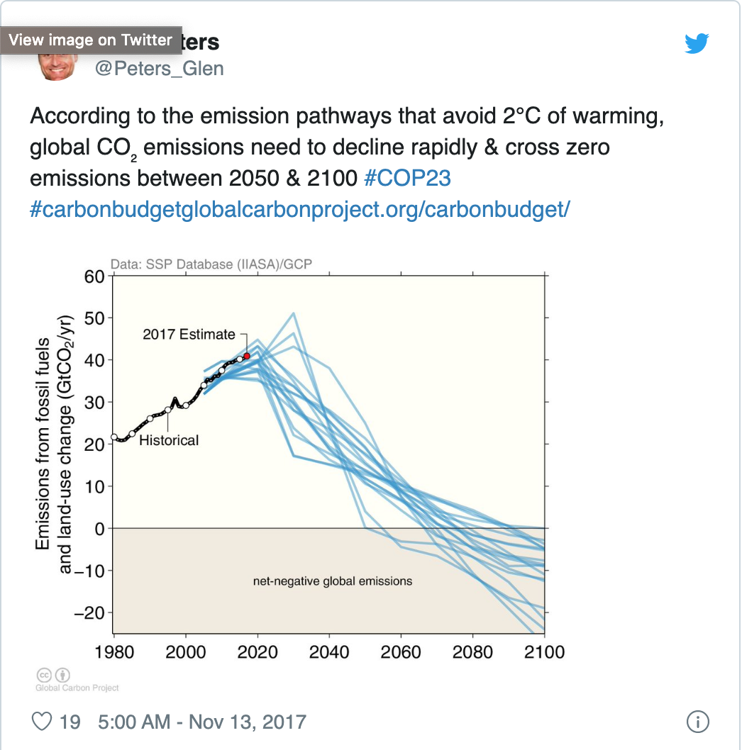
https://twitter.com/Peters_Glen/status/930042574777257984
(Arguably, talking about “net zero” is too vague and we should instead have separate, definite targets for both positive and negative emissions.)
The need for a (revenue-neutral, staged) carbon tax
How can this change be incentivized? There are powerful arguments in favor of a carbon tax. Specifically, one can do a gradually scaled-up, revenue-neutral carbon tax that would, for instance, return the revenues back to consumers as rebates or tax reductions in other kinds of taxes — this could be important as almost any form of carbon tax would ultimately be passed at least in significant part onto the consumer, and many consumers are cash-strapped already, e.g., struggling to afford gas for their commute.
How big a carbon tax, and what effects would that have on citizens? That’s a complicated question and not one I have found a full answer to. Typical values suggest something like $10-$100 per tonne of CO2, meant to offset widely-varying estimates of the social cost of carbon. That would apparently increase, say, the gas bill for your car by roughly 10 cents to 1 dollar per gallon of gas (the current average price of gas in the USA is around $2.50/gallon, and there is already an excise tax on it of about 1/10 that).
Alas, consumers in the USA seem wary of changes in that range. It is unclear if they would still be wary if they were presented with a rebate (remember, the carbon tax can be revenue-neutral, or at least with significant offsets to give cash back to citizens, although some would hope to use revenues from a carbon tax to fund climate-related programs and deployments) that would on net leave most people’s bank accounts the same or fatter, not thinner.
A few points of comparison:
- We’ll see in the next post that technologies aiming to scrub carbon from the atmosphere are shooting to get their cost of CO2 produced into this same range, say <$100/tonne CO2.
- If the US is currently emitting 6 GigaTonnes of CO2 and we had a $40/tonne CO2 carbon tax right now, that would presumably be something like $240 billion per year in carbon tax revenue, or a bit under 1/10 of all US federal tax revenue of $3.something trillion. Could we re-structure the rest of the tax code to give back 1/10 to consumers, as a rebate, so that their bank accounts (and the overall size of government) stay roughly flat? I bet we could. But this puts into perspective that, if someone is instead talking about a $400/tonne CO2 price of carbon (see the Stern Review item in the table below), that’s approaching the totality of all other tax revenue in the USA at current emissions levels.
- That $240 billion paid against the $40/tonne carbon price is around 1.2% of US GDP of around $20 trillion.
There are also some arguments against a carbon tax, e.g., that a carbon tax in the US doesn’t impact other countries like China and may simply shift international trade balances, or that they might be revoked, as well as the need for them to be sufficiently large and thus correspondingly painful to the consumer in order to make a difference. They are also empirically not easy to pass, and economists are studying why.
France had a fuel tax of about $60/ton CO2 equivalent, but when Macron tried to double that over the next 4 years, the Yellow Vest protests happened (this may of course be specific to the kind of fuel tax they imposed and the particular situation there). Canada did pass a carbon tax starting at below that level and rising to near it over a few years (“start low at $20 per ton [tonne of emitted CO2] in 2019, rising at $10 per ton per year until reaching $50 per ton in 2022”). Recently, some major fossil energy companies started lobbying in favor of a carbon tax, which I found surprising — alas, it looks like they are putting in pennies compared to their fossil-fuel-promoting endeavors, in a bid to insure themselves against future climate-related lawsuits!
Cap and trade is another possibility, arguably fundamentally similar. Cap and trade has the advantage of directly setting a specific emissions limit. China has established something of a cap and trade system. It doesn’t look that stringent, yet: “The scheme set the initial carbon allowances to 3–5 billion tonnes per year.”
Subsidizing R&D into decarbonization technologies is the key alternative suggested by Noah Smith — if you get a breakthrough towards lower-cost technology, that can be adopted anywhere in the world (including places that may not feel they can afford a carbon tax), and only benefits people (no change in tax structure). We obviously need that too, big time. This thread has a coherent discussion about why carbon taxes can help to scale existing technologies but, for areas where truly new technologies are needed (of which there are many), targeted R&D and highly specific subsidies can be better.
Before we finish this first post, let’s take a look at how economists estimate how big a carbon tax we really should have? Consider this snippet from the Nobel Prize announcement for economist William Nordhaus, who pioneered this area:

https://www.nobelprize.org/uploads/2018/10/popular-economicsciencesprize2018.pdf
Nordhaus uses coupled climate + economic activity and growth models to evaluate “optimal” scenarios — ones with the maximum overall growth in the economy, factoring in the effects of damage from climate change and the costs of introducing decarbonization approaches. His optimal overall economic scenario (“Opt”) is the one shown in red in the plot above, with a global carbon tax starting at $30-40/tonne CO2 or so (and rising to about $50/tonne by 2030 and then further afterwards, see table below). Note, though, that this pathway massively overshoots the orange and black pathways in terms of emissions — the black and orange pathways look more like the other graphs we’ve seen for full decarbonization by 2050. Here is a table from his 2017 PNAS paper with a comparison:

Proceedings of the National Academy of Sciences 114.7 (2017): 1518-1523.
Nordhaus, William D. “Revisiting the social cost of carbon.”
Proceedings of the National Academy of Sciences 114.7 (2017): 1518-1523.
Indeed, the optimality of an Opt-like pathway is a subject of great controversy. Nordhaus’s “optimal” carbon pricing, in that model, would get us to a temperature rise of 3.5C (!) or so from preindustrial, while pushing to full decarbonization by 2050, in order to stay below 2C, would require roughly an order of magnitude higher carbon price. Staying below 1.5C would seem, according to such models, to imply a need for even higher carbon prices. From a recent review:

Annual Review of Environment and Resources. 2018 Oct 17;43:455-80.
Dietz S, Bowen A, Doda B, Gambhir A, Warren R. The economics of 1.5 C climate change.
Annual Review of Environment and Resources. 2018 Oct 17;43:455-80.
Now, obviously, if Nordhaus’s model had included, say, Antarctica completely melting and many major cities going completely underwater due to a series of major sea ice and other tipping points being crossed, the social cost of carbon would need to be a lot higher. So implicitly the risk of such scenarios is considered low in such models. At a more subtle level, the particulars of these optima depend on the expected cost of decarbonization (which depends on the rate of technological innovation), on the temporal discount rates used (you can see in the table above that prices rapidly rise with decreasing discount rate), and on other factors.
There are some good-sounding arguments for having carbon prices instead start high, and then decline, political difficulties notwithstanding — I haven’t understood the full details, but this approach seems to focus on mitigating risk and to take into account more of the variance in scenarios and our finite but improving knowledge thereof.
The fact is, as the Nobel Prize announcement notes, there are huge uncertainties in what would really be optimal (even within the philosophical frame that underlies Nordhaus’s analysis, e.g., with the type and rough magnitude of the discount rate he uses, and even neglecting the politics of passing such taxes) — it depends on the cost of decarbonizing quickly, and on the climate damage cost of not decarbonizing quickly, both of which are highly uncertain at present. So we have to take a best guess — but that best guess should incorporate the uncertainty.
This brings us back to the role of technology: it can reduce the cost of decarbonization, and it can mitigate tail risks from climate damage. Advanced technology is crucial to allow us to decarbonize safely and quickly, with minimal economic cost. It allows a lower self-imposed carbon price to have greater benefit, shifting the estimated-to-be-economically-optimal pathways to overlap those that strongly limit the risk of crossing catastrophic climate tipping points.
Tentative conclusions
My sense — again, as an outsider to the field simply trying to grok the literature in my free time — is that we should do the following:
- Make sure our ability to measure and model everything in the climate system continues to improve, including for complex land and ocean biological effects.
- Lobby for a revenue-neutral, staged price on carbon, in rich countries initially — rich countries can bring down the cost for poor countries by developing and scaling up better, cheaper technology. In the USA there is a specific program with some high-profile advocates called the Carbon Dividends Plan. I certainly don’t want to say that a carbon tax is the only necessary policy though — also advanced R&D, tax credits, subsidies, lobbying reform, and down the line hopefully new social technology for making societal decisions would come into play.
- Economically incentivize a full transition to net-negative emissions by around 2050. This includes deploying a portfolio of existing clean technologies now to limit our cumulative carbon emissions and peak CO2 concentration.
- Heavily invest in large-scale, advanced R&D to bring down the cost of grid-scale energy storage, next-generation nuclear, novel clean manufacturing processes for things like steel and cement, improved agricultural technologies, smart grid-integrated buildings, and synthetic meat (among other areas). With enough technological innovation, I hope that the cost to decarbonize could be brought lower than the estimates of those like Nordhaus.
- Heavily invest in sustainable land use management and conservation, as well as aggressive afforestation.
- Switch to electric cars. (This will impact multiple key areas.)
- Bootstrap the nascent fields of direct air carbon capture / carbon sequestration, both chemical and biological, to the point where they can really scale cost-effectively (next post), and seriously consider ocean liming, sequestration of agricultural waste biomass, and so forth (also next post). This involves both new research and the creation of new markets for carbon. Use sequestered carbon to make the jet fuel.
- Do the fundamental R&D on emergency adaptation strategies like solar radiation management and buttressing of glaciers (next next post).
You can go to the next post on negative emissions.
5 comments
Comments sorted by top scores.
comment by jimrandomh · 2019-10-29T01:37:06.391Z · LW(p) · GW(p)
I expect to have some questions and ideas, but I'm still working my way through this, as I suspect are others. I really appreciate how in depth this is!
comment by jimrandomh · 2019-10-29T03:07:07.098Z · LW(p) · GW(p)
Nuclear power is typically located close to power demands, ie cities, because of the costs and losses in transporting power over long distances. This also limits the size/scale of nuclear power plants, since if you build larger than the demands of a city, you have to transport the power over a long distance to find more sinks.
On the other hand, suppose a city were built specifically for the purpose of hosting nuclear power, carbon-capture, and CO2-to-fuel plants. Such a city might be able to have significantly cheaper nuclear power, since being far away from existing population centers would lower safety and regulatory costs, and concentrating production in one place might enable new economies of scale.
It seems like there are two worlds we could be in, here. In one world, nuclear power right now is like the space launch industry of a decade ago: very expensive, but expensive because of institutional failure and a need for R&D, rather than fundamental physics. In the other world, some component of power plants (steam turbines, for example) is already optimized close to reasonable limits, so an order of magnitude is not possible. Does anyone with engineering knowledge of this space have a sense of which is likely?
comment by jimrandomh · 2019-10-29T02:11:38.054Z · LW(p) · GW(p)
Something that confuses me. This (and also other) discussions of afforestation focus on planting trees (converting non-forest biomes into forest). But it seems like trees do a reasonably good job of spreading themselves; why not instead go to existing forests, cut down and bury any trees that are past their peak growth phase, and let the remaining trees plant the replacements? How much does the cutting and burial itself cost? (I see an estimate of $50/t for burying crop residues, which seems like it would be similar.)
comment by waveman · 2019-11-12T02:02:11.153Z · LW(p) · GW(p)
Excellent post.
One oversight I see often in this space, and here, relates to a carbon tax. It is stated that the revenue from a carbon tax can be used to compensate people, especially lower income people, for the increased cost of living resulting from the tax. The fatal problem with this is that in a zero emissions world, there will be no emissions and therefore no carbon tax revenue.
Of course it may be possible to compensate people via other means such as other taxes. But a carbon tax is only required because it is otherwise cheaper to emit carbon. This means costs will go up overall and that there will be a net loss (in the short term at least). There is no free lunch and someone will have to pay.
comment by B Jacobs (Bob Jacobs) · 2020-06-22T22:32:31.430Z · LW(p) · GW(p)
Just wanted to add a link to the newest carbon capture plant that could suck out as much carbon dioxide as 40 million trees. Backed by Bill Gates this plant can capture one ton of co2 for less than $233.