Calibration for continuous quantities

post by Cyan · 2009-11-21T04:53:32.443Z · LW · GW · Legacy · 13 comments

Contents

  It's the PITs
  Take-home message
None
13 comments

Related to: Calibration fail, Test Your Calibration!

Around here, calibration is mostly approached on a discrete basis: for example, the Technical Explanation of Technical Explanations talks only about discrete distributions, and the commonly linked tests and surveys are either explicitly discrete or offer only coarsely binned probability assessments. For continuous distributions (or "smooth" distributions over discrete quantities like dates of historical events, dollar amounts on the order of hundreds of thousands, populations of countries, or any actual measurement of a continuous quantity), we can apply a finer-grained assessment of calibration.

The problem of assessing calibration for continuous quantities is that our distributions can have very dissimilar shapes, so there doesn't seem to be a common basis for comparing one to another. As an example, I'll give some subjective (i.e., withdrawn from my nether regions) distributions for the populations of two countries, Canada and Botswana. I live in Canada, so I have years of dimly remembered geography classes in elementary school and high school to inform my guess. In the case of Botswana, I have only my impressions of the nation from Alexander McCall Smith's excellent No. 1 Ladies' Detective Agency series and my general knowledge of Africa.

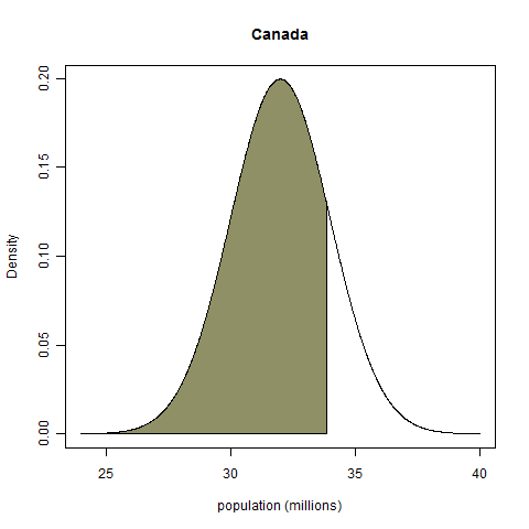
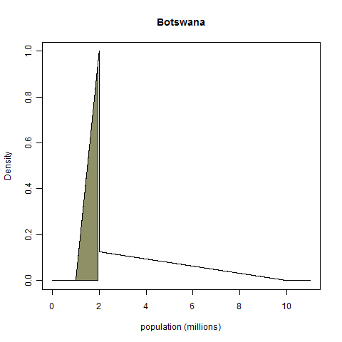
For Canada's population, I'll set my distribution to be a normal distribution centered at 32 million with a standard deviation of 2 million. For Botswana's population, my initial gut feeling is that it is a nation of about 2 million people. I'll put 50% of my probability mass between 1 and 2 million, and the other 50% of my probability mass between 2 million and 10 million. Because I think that values closer to 2 million are more plausible than values at the extremes, I'll make each chunk of 50% mass a right-angle triangular distribution. Here are plots of the probability densities:

 

(These distributions are pretty rough approximations to my highest quality assessments. I don't hold, as the above normal distribution implies, that my probability that the population of Canada is less than 30 million is 16%, because I'm fairly sure that's what it was when I was starting university; nor would I assign a strictly nil chance to the proposition that Botswana's population is outside the interval from 1 million to 10 million. But the above distributions will do for expository purposes.)

For true values we'll take the 2009 estimates listed in Wikipedia. For Canada, that number is 33.85 million; for Botswana, it's 1.95 million. (The fact that my Botswana estimate was so spot on shocked me.) Given these "true values", how can we judge the calibration of the above distributions? The above densities seem so dissimilar that it's hard to conceive of a common basis on which they have some sort of equivalence. Fortunately, such a basis does exist: we take the total probability mass below the true value, as shown on the plots below.

No matter what the shape of the probability density function, the random variable "probability mass below the realized value" always has a uniform distribution on the interval from zero to one, a fact known as the probability integral transform¹. (ETA: This comment gives a demonstration with no integrals.) My Canada example has a probability integral transform value (henceforth PIT value) of 0.82, and my Botswana example has a PIT value of 0.45.

It's the PITs

If we have a large collection of probability distributions and realized values, we can assess the calibration of those distributions by checking to see if the distribution of PIT values is uniform, e.g., by taking a histogram. For correctly calibrated distributions, such a histogram will look like this:

 

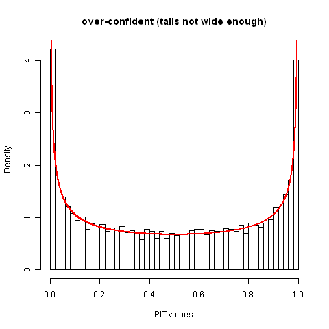
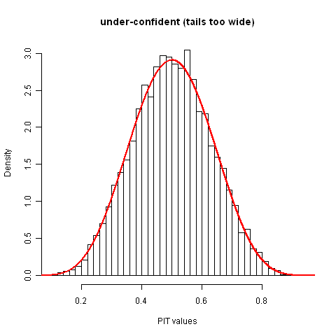
The above histogram and the ones below show 10,000 realizations; the red line gives the exact density of which the histogram is a noisy version.

Figuring out that your distributions are systematically biased in one direction or another is simple: the median PIT value won't be 0.5. Let's suppose that the distributions are not biased in that sense and take a look at some PIT value histograms that are poorly calibrated because the precisions are wrong. The plot below shows the case were the realized values follow the standard normal distribution and the assessed distributions are also normal but are over-confident to the extent that the ostensible 95% central intervals are actually 50% central intervals. (This degree of over-confidence was chosen because I seem to recall reading on OB that if you ask a subject matter expert for a 95% interval, you tend to get back a reasonable 50% interval. Anyone know a citation for that? ETA: My recollection was faulty.)

I wouldn't expect humans to be under-confident, but algorithmically generated distributions might be, so for completeness's sake I'll show that too. In the case below, both the assessed distributions and the distribution of realized values are again normal distributions, but now the ostensible 50% intervals actually contain 95% of the realized values.

Take-home message

We need not use coarse binning to check if a collection of distributions for continuous quantities is properly calibrated; instead, we can use the probability integral transform to set all the distributions on a common basis for comparison.

¹ It can be demonstrated (for distributions that have densities, anyway) using integration by substitution and the derivative of the inverse of a function (listed in this table of derivatives).

13 comments

Comments sorted by top scores.