How does a toy 2 digit subtraction transformer predict the sign of the output?

post by Evan Anders (evan-anders) · 2023-12-19T18:56:22.487Z · LW · GW · 0 comments

This is a link post for https://evanhanders.blog/2023/12/15/2-digit-subtraction-how-does-it-predict/

Contents

  Summary
  Intro
  Mathematical Framework
  Working Backwards: Logits
  Logit-Neuron Connection
  Working Backwards: Neuron Activations
  Embedding-Neuron connection
  Attention Patterns
  What about biases?
  The algorithm
  Wrap Up
  Code
  Acknowledgments
None
No comments

 

Summary

I examine a toy 1-layer transformer language model trained to do two-digit addition of the form $a-b=\pm c$. This model must first predict if the outcome is positive (+) or negative (-) and output the associated sign token. The model learns a classification algorithm wherein it sets the + token to be the default output, but when $b>a$ the probability of the - token linearly increases while the probability of the + token linearly decreases. I examine this algorithm from model input to output.

Intro

In my previous post (which was a whole week ago before I knew about lesswrong!), I briefly discussed a 1-layer transformer model that I've trained to do two-digit subtraction. The model receives input of the form $a-b=$ and has to predict the sign of the result ($\pm$) and the numerical value (so e.g., in $46-16=+30$, it would have to predict + and 30). In this blog post, I'll investigate the algorithm the model uses to predict if the sign should be positive or negative.

Mathematical Framework

I'm once again being inspired by the Chapter 1, part 5 ARENA notebook on understanding modular addition. The action of the transformer to produce the logits $\ell$ can be described by the following equation:

$\ell =\text{ReLU}\left(\left[{\sum }_h{A}^h{x}_0{W}_{OV}^h\right]W_{in}\right)W_{out}{W}_U.$

Here, $\text{ReLU}$ is the Rectified Linear Unit activation function, $x_0$ is the residual stream values after embedding (accounting for positional and token embedding), $W_{in}$ and $W_{out}$ are the input and output matrices for the MLP, $W_U$ is the unembedding matrix, $W_{OV}^h=W_V^h{W}_O^h$ is the output-value matrix constructed of the output and value weights in head $h$, and the attention pattern of head $h$ is $A^h=\text{softmax}\left(\frac{x_0{W}_Q^h(W_K^h{)}^T{x}_0^T}{\sqrt{d_{head}}}\right)$, constructed from the residual stream and the query and key weights. In the above equation I've made the following simplifying assumptions:

• The direct logit contributions from the attention output and from the direct embedding are negligible compared to the output of the MLP. (I've verified this is the case.)
• The bias terms are unimportant. (I'll show later that this is not quite the case, but they just provide constant offsets to the + and - logits. Here I'm interested in how the logits respond to different inputs in the vocabulary!)

Working Backwards: Logits

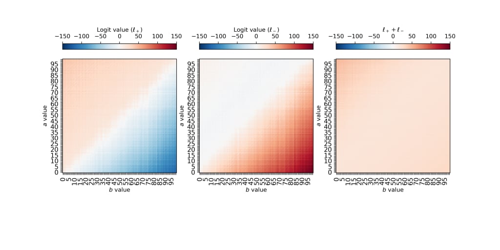
In our problem, our sequence length is 6 (four inputs, 2 outputs). The fourth spot (Python index 3) in the sequence corresponds to the = token, and is the location in the sequence where the model predicts if the output is positive or negative. At index 3 in the sequence, let's look at the logit values for the + token and the logit values for the - token:

So we see that the + logit (left panel, ${\ell }_{+}$) has a moderate value of $\sim 20$ for values where $a>b$, and seems to decrease linearly to the bottom right corner where $b\gg a$. On the other hand, the - logit (middle panel, ${\ell }_{-}$) looks to have a roughly constant value of $\sim$ 0 when $a>b$, and increases linearly toward the bottom right corner. If we add these two logit values together (right panel), the increasing feature in the bottom right corner disappears -- so these are roughly equal and opposite.

Great. This seems really comprehensible. Let's go a step backward. The logits can be computed from the neuron activations by multiplying the matrix $W_{logit}=W_{out}{W}_U$. Let's look at some activations.

Logit-Neuron Connection

The matrix $W_{logit}$ has shape (d_mlp, d_vocab). A single row of this matrix (e.g., W_logit[0,:]) corresponds to how much a given neuron boosts each logit.

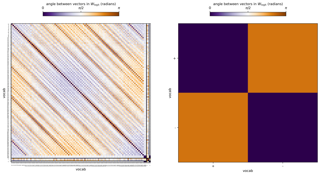
One thing I'm particularly interested in is the angle between the vectors in this space. That is, how does the vector corresponding to logit boosts for the + token (W_logit[:,100]) relate to the logit boosts for the - token (W_logit[:,101])? I've computed the angle between the vectors for every pair of tokens in the vocabulary:

Above, the left panel shows the angles between each vector and each other vector (so the top row is the angle between 0 and every other token along the x-axis, for example). Dark purple means the vectors are aligned, dark orange means they're anti-aligned, and white means they're perpendicular. The diagonal is purple definitionally, but it's interesting that most of the numbers are at least partially aligned with one another.

In the left panel I zoom in on the bottom right corner where the plus and minus tokens are compared. We see that these tokens are strongly anti-aligned (with an angle of $\sim 0.83\pi$ between them). This means that a neuron that boosts the + token will throttle the - token at the same time (and vice-versa). This makes sense given the patterns seen above -- the + logits decrease where the - logits increase. And most of the neurons that I find to be important in the next section simultaneously boost the - logit while decreasing the + logit in the bottom right corner of the plot I showed in the first figure in this post.

Working Backwards: Neuron Activations

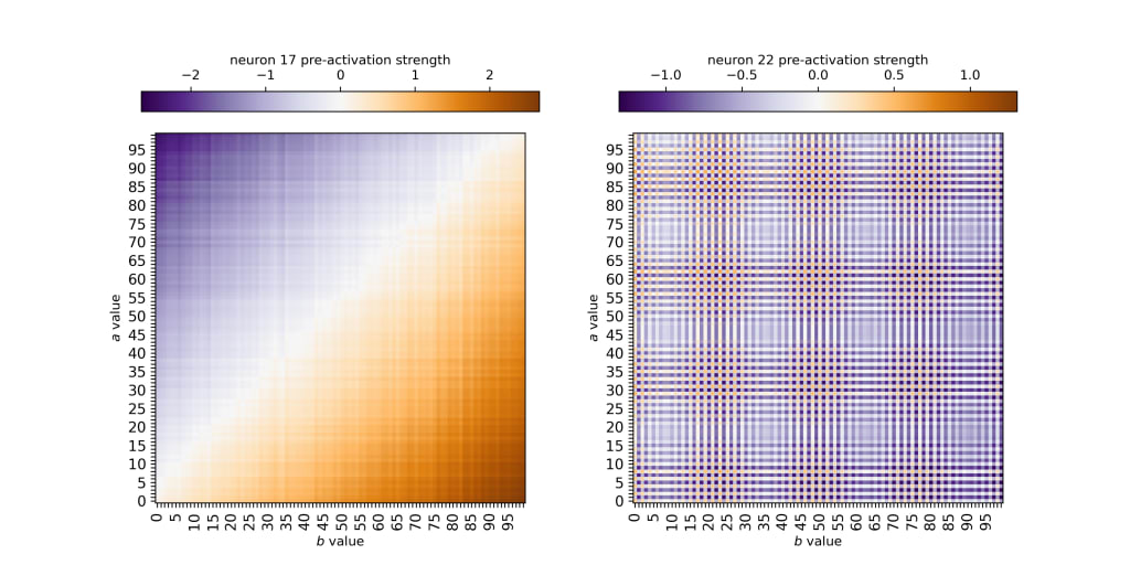
Next I'm looking at neuron activations and pre-activations. There seem to be two predominant important classes of neurons in this problem, and a sample from each class is shown below:

On the left (neuron 17) we see a very similar pattern compared to the logit patterns we saw above, with the neuron pre-activation strength increasing towards the bottom right ($b>a$) and decreasing towards the upper left ($a>b$). On the right we see a neuron with strong periodicity in its activation, which are probably important for outputting the proper number but not the $\pm$ sign, so we'll just focus on the pattern on the left for now.

I also want to briefly note that many neurons are somewhat polysemantic -- they contain both the linear and oscillatory features shown above. This isn't surprising but let's ignore it for now.

The preactivation of neuron $i$ for neurons like neuron 17 can be largely described in terms of a simple linear function  $n_i(a,b)=c_1(a-b)+c_2$. for constants $c_1,c_2$. I use SciPy's curve_fit function to fit this simple function of  $n_i(a,b)$ for each neuron. For neurons like the one on the right in the above image, I unsurprisingly find  $c_1\approx 0$, whereas for e.g., the one on the left I find  $c_1=-0.024$ and  $c_2=0.126$. This is a big enough slope to cause $O\left(1\right)$ changes across parameter space.

I define the neurons that are important to the $\pm$ calculation as the neurons where $|c_1|>{10}^{-3}$ -- this means the preactivation varies by $O\left(0.1\right)$ across parameter space, and 270/512 neurons cross this threshold. If I zero ablate these neurons, loss on the $\pm$ prediction increases from 0.068 to 3.79 and accuracy decreases from 98.5% to 12.7%. If I ablate the remaining 242 neurons but keep these neuron activations, then loss on the $\pm$ prediction only increases from 0.068 to 0.069 while accuracy decreases from 98.55 to 98.53.

Further, if I replace ALL neuron pre-activations with just a best-fit to the simple linear function from above, the loss only increases from 0.068 to 0.080 and accuracy only decreases from 98.5% to 97.93%. So I feel reasonably confident saying that the algorithm used to predict $\pm$ uses the attention and input MLP operations to create these linear functions.

Embedding-Neuron connection

Next we examine how token embeddings connect to the neurons. I'm currently looking at this in a way that's agnostic to attention pattern. I'm interested right now in how the attention heads contribute to the neurons assuming that the attention head attends to a token.

This is described, for each attention head, by the matrix $W_{neur}^h=W_E{W}_V^h{W}_O^V{W}_{in}$. This matrix has the shape [d_vocab, d_mlp], so if I want to understand how each token in the vocabulary affect a neuron, I just have to index the right column of this matrix.

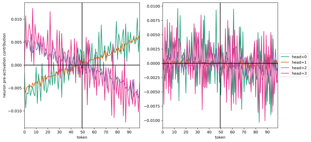
Here are the contributions of the attention heads to the two neurons (17 and 22) that I showed previously:

So we see that heads 1 and 2 make a predominantly linear contribution to the neuron pre-activations with little variance, while heads 0 and 3 contribute with a lot of high-frequency oscillations on top of a linear trend. For one of the neurons that's important to the $\pm$ token (neuron 17, on the left), all four attention heads have a strong linear trend, and heads 0 and 1 share a slope which is opposite that of heads 2 and 3. On the right (a periodic but not important neuron for the $\pm$ token), we see that the signal is basically purely oscillatory.

To quantify this a bit: a linear polynomial fit for neuron 17 accounts for 68%, 97%, 89%, and 53% for heads 0, 1, 2, and 3 respectively and the slopes and intercepts of e.g., head 0 and head 3 are basically equal and opposite. Meanwhile a linear fit accounts for <5% of all variance for all heads for neuron 22.

So when a token is attended to, it maps its value in this linear function onto the neuron in a function of the form:

$n_i(a,b)={\sum }_h\left(A_{h,a}\right(m_{h,i}a+o_{h,i})+A_{h,b}(m_{h,i}b+o_{h,i}\left)\right),$

where $A_{h,a}$ and $A_{h,b}$ are how strongly head $h$ attends to tokens $a$ or $b$, $m_{h,i}$ is the slope of the linear fit head $h$ contributes to neuron $i$, and $o_{h,i}$ is the y-intercept of the linear fit of the contribution of head $h$ to neuron $i$.

Great. Now we just need to figure out what $A_{h,a}$ is, and we're ready to construct the algorithm behind the full $\pm$ classification.

Attention Patterns

The attention pattern is constructed from the queries and keys in the attention layer, and takes the form $A^h=\text{softmax}\left(\frac{x_0{W}_Q^h(W_K^h{)}^T{x}_0^T}{\sqrt{d_{head}}}\right)$. Before the softmax is applied, an autoregressive mask is applied, so that any token position can only pay attention to the present token and past tokens, but not to future tokens. So when our transformer comes to the = sign, it can self-attend, and it can attend to $a$ and $b$ (it can also attend to -, but ablating the - position after embedding causes essentially no change in loss). The attention pattern has shape [batch, n_heads, n_seq, n_seq], and has values between 0 and 1. If, for example, the [10, 2, 3, 0] value is large (1), then that means, for the data sample at index 10 in the batch, at the sequence position of the = sign (3), attention head 2 attends to position 0 ($a$).

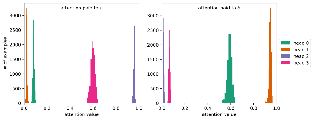
Here are histograms of how strongly each attention head attends to $a$ and $b$:

We see that head 1 always attends to $b$ and never $a$; likewise head 2 always attends to $a$ and never $b$. Heads 0 and 3 are more confusing, but they also have a similar paired behavior -- head 0 attends somewhat strongly (0.6) to $b$ and weakly (0.1) to $a$, whereas head 3 is the reverse. The attention pattern must sum to 1, and heads 0 and 3 split the remaining attention $\sim 0.3$ evenly between position 1 (the - sign) and position 3 (the = sign) -- which means these heads are involved in an overall bias to the system, which I hope to explore later.

But -- great! A decent approximation for our model is to say that $A_{h,a}\approx [1,0.6]$ for heads 2 and 3 (with $A_{h,b}\approx [0,0]$ for heads 0 and 1), and to say $A_{h,b}\approx [1,0.6]$ for heads 1 and 0 (with  $A_{h,b}\approx [0,0]$ for heads 2 and 3).

*If* all important neurons are like neuron 17 (look a couple images ago), then we can also note that the contributions of  $b$ from heads 0 and 1 to the neuron will be equal and opposite to those from $a$ from heads 2 and 3. So we can approximate the neuron contributions:

 $n_i(a,b)={\sum }_h^{0,1}{A}_{h,b}\left(m_{h,i}\right(b-a)+o_{h,i})$.

Where for this equation I have adopted the convention that $m_{0,i}=m_{3,i}$ and $m_{1,i}=m_{2,i}$, and I've wrapped the opposite-ness in the sign of $a$.

What about biases?

So far I've only focused on what the model does with token-dependent information, not what the model does with information from all of the biases. To figure this out, we just need to zero-ablate the token embedding of $a$ and $b$. Doing so increases loss by about a factor of 100 on the $\pm$ token, but accuracy only decreases to 50.5%!

This is not surprising. The biases set the baseline logit value of the + token to 18.6 and the baseline logit value of the - token to 6.21. So without information about the tokens, the model assumes that the + token is the right prediction after the = sign. Since I've set up my values to list 0 as a positive value (e.g., $50-50=+0$), 50.5% of all possible inputs will start with a + sign, so the model hedges and makes that the default.

The algorithm

The model generates a classification algorithm that is roughly of the form:

\$el{l}_{+}\approx \{\begin{array}{cc}{b}_{+}& a\ge b\\ b_{+}-m(b-a)& a<b\end{array},{\ell }_{-}\approx \{\begin{array}{cc}{b}_{-}& a\ge b\\ b_{-}+m(b-a)& a<b\end{array}$,

where ${\ell }_{\pm }$ are the logit values, $b_{\pm }$ are the results of biases, and $m>0$ is a constant slope.

The model achieves this by constructing neuron pre-activations (for neuron index $i$) of the form

 $n_i(a,b)={\sum }_h^{0,1}{A}_{h,b}\left(m_{h,i}\right(b-a)+o_{h,i})$,

where $A_{h,b}\approx 1$, and then the model uses the ReLU activation to zero out any trends for the part of parameter space where $a>b$ before mapping (in opposite directions) to the logits. In other words, the model learns to determine if the outcome is negative, but doesn't really pay any attention to whether or not it's positive; it just assumes that as a default.

Wrap Up

Ok! I feel like I have a good handle on how to walk from logits back through the model to determine if the outcome is positive or negative. I didn't see it at first but of course this is just a classification task! In the next post (hopefully before Christmas break...), I'll need to figure out how the model predicts the outcome number, which is a regression task.

Code

The code I used to train the model can be found in this colab notebook, and the notebook used for this investigation can be found on Github.

Acknowledgments

Big thanks to Adam Jermyn for helping me find my footing into AI safety work and for providing me with mentorship and guidance through this transition and this project. Also thanks to Adam for suggesting I cross-post to lesswrong! I'd also like to thank Philip Quirke and Eoin Farrell for meeting regularly and providing me with a community as I'm skilling up in the field.

0 comments

Comments sorted by top scores.