Measuring Learned Optimization in Small Transformer Models

post by J Bostock (Jemist) · 2024-04-08T14:41:27.669Z · LW · GW · 0 comments

Contents

  Methods
    Pretraining on Sequence Prediction
    Measuring Optimization
  Results
    Optimization vs RL Success Rate
    Cross-Objective Evaluation
    Optimization vs Impact
    Model Self-Evaluation
  Conclusions
      Alex Turner's Existing Work
  Appendices
    Appendix A: Impact and Differential Impact
      Derivation of Imp
      Differential Impact
    Appendix B: Proofs
      Derivation and proof of Imp≥Impmin
      Derivation of Differential Impact
      Derivation of Multivariate Differential Impact and Optimization
    Appendix C: Supplementary Plots
      Other Ways to Visualize Impact Plots
      Example training runs from ngood = 4
      Example figures summarizing training runs:
None
No comments

This is original, independent research carried out in March and April of 2024.

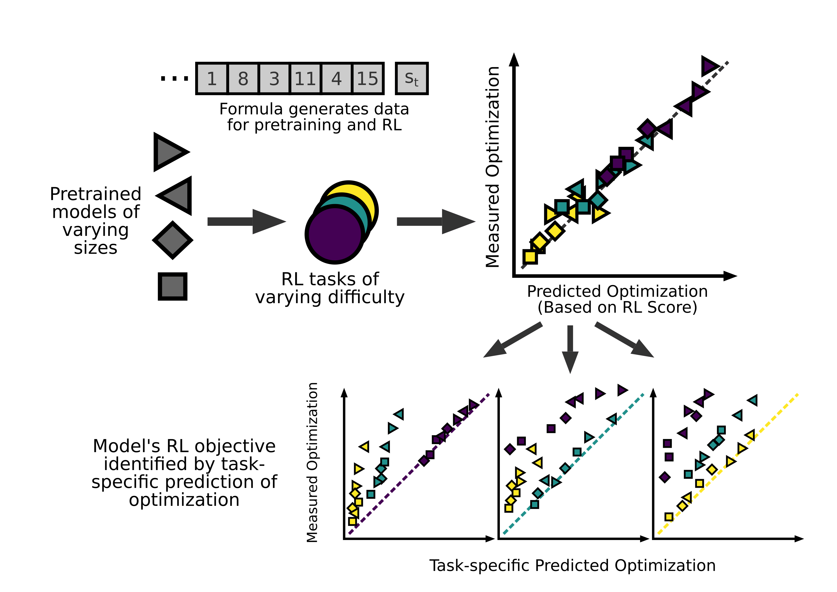
The degree to which a a policy optimizes the future can be quantified mathematically. A set of of very small transformer models were pretrained to predict the next token in a mathematical sequence, then subjected to reinforcement learning finetuning.

The optimizing power of each model can be predicted with high accuracy based on each model's score on its own RL task. By comparing predictions of optimization based on scores on each different RL task, a model's original reinforcement objective can be identified.

A related measure for impact can also be derived mathematically, and given a theoretical lower bound based on RL score. This gives further information about model behavior, and allows for the same analysis as the measure of optimization.

I also investigate the possibility of getting models to self-evaluate optimization and impact, with limited success.

Methods

Pretraining on Sequence Prediction

I defined a simple mathematical sequence defined by the following stochastic recurrence relation. This produces a pseudo-random but (to 98%) predictable sequence, alternating between elements of $\{0,...,7\}$ on even values of $t$ and $\{8,...,15\}$ on odd values of $t$.

$s_t=(\{\begin{array}{cc}\left(\right(\stackrel{16}{\prod _{i=1}}(s_{t-i}+1)\mathrm{mod}17\left)\mathrm{mod}8\right)& \text{with probability 98\%}\\ \in \{0,...,7\}& \text{with probabiltiy 2\%}\end{array})+8\times \left(t\mathrm{mod}2\right)$

I then trained a small encoder-only transformer model to predict the next element in the sequence given the previous 20 elements of the sequence.

This was followed by a reinforcement-learning phase in which the transformer was used to generate the next token on odd values of $n$ only, and the recurrence relation was used to generate the value of $s_{t+1}$. If $s_{t+1}$ was in $\{0,2,4,6\}$, this was used as a "successful" example to reinforce the model. I used a temperature of 1 when generating these sequences to introduce some randomness, but the temperature was reduced to 0 during evaluations and when calculating optimization.

A small amount of "maintenance" training (much lower learning rate) was used during this phase to ensure that model performance on the predictive tasks for even values of $t$ was maintained. Without this I saw rapid loss of performance on the "maintenance" dataset. I also found that I was unable to include "unsuccessful" examples (i.e. where $s_{t+1}\notin \{0,2,4,6\}$) with even a tiny negative learning rate, as this caused worsened performance at all tasks. Here is a typical set of results from training and evaluation:

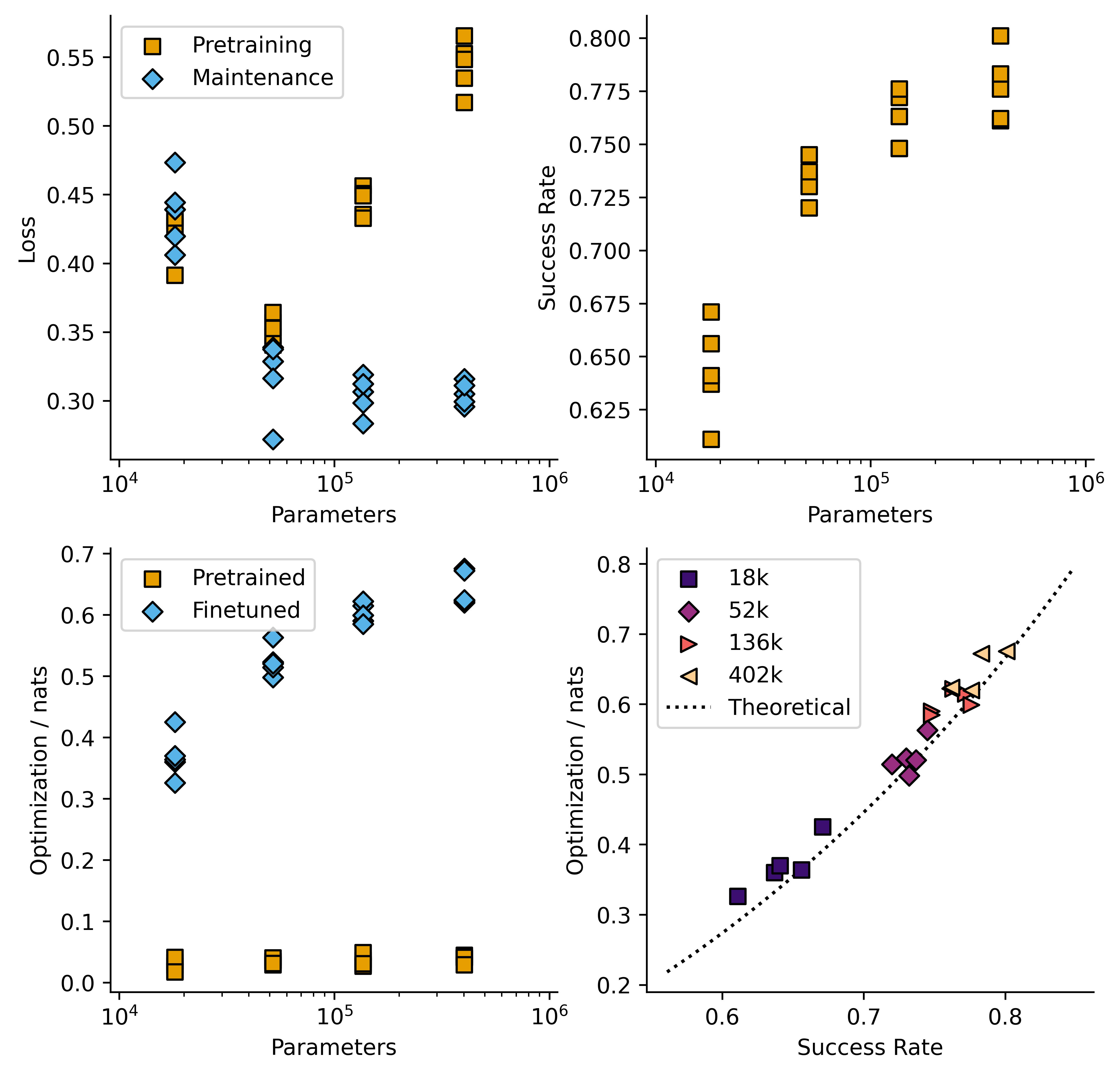
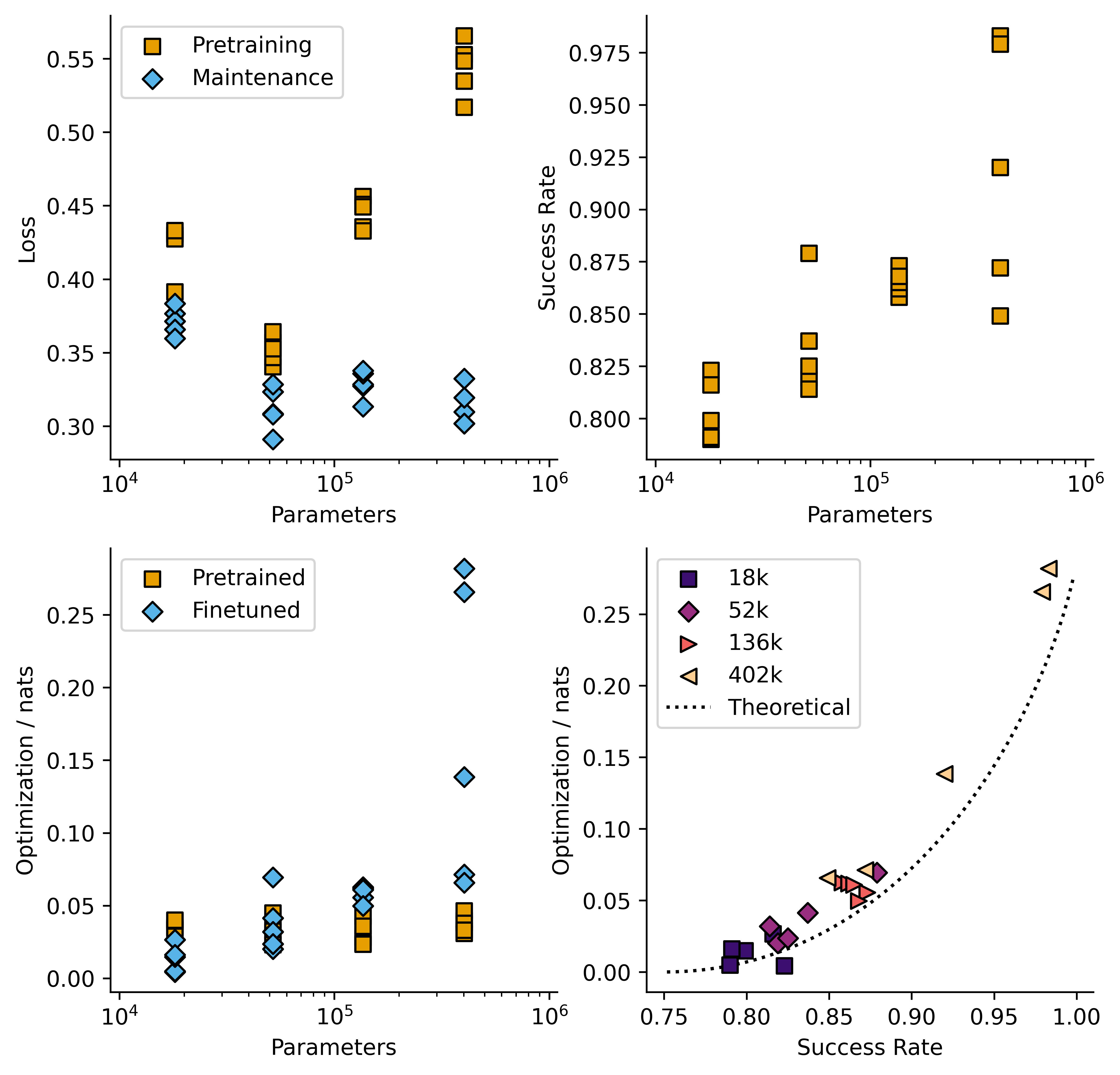
I carried out this training on $N=5$ models per size for four model sizes between 18k and 402k parameters, giving the following plot:

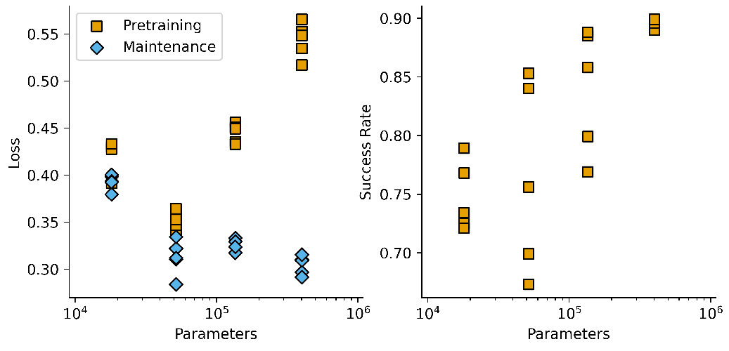
Pretraining loss increases over the last few model sizes, and the loss/time plots (some of which I have put in the Supplementary Information at the bottom of this post) showed signs of overfitting in the large models. Regularization was employed during training (0.01 weight decay in an AdamW optimizer, 10% dropout rate for neurons) so perhaps a larger dataset size is required to totally avoid this.

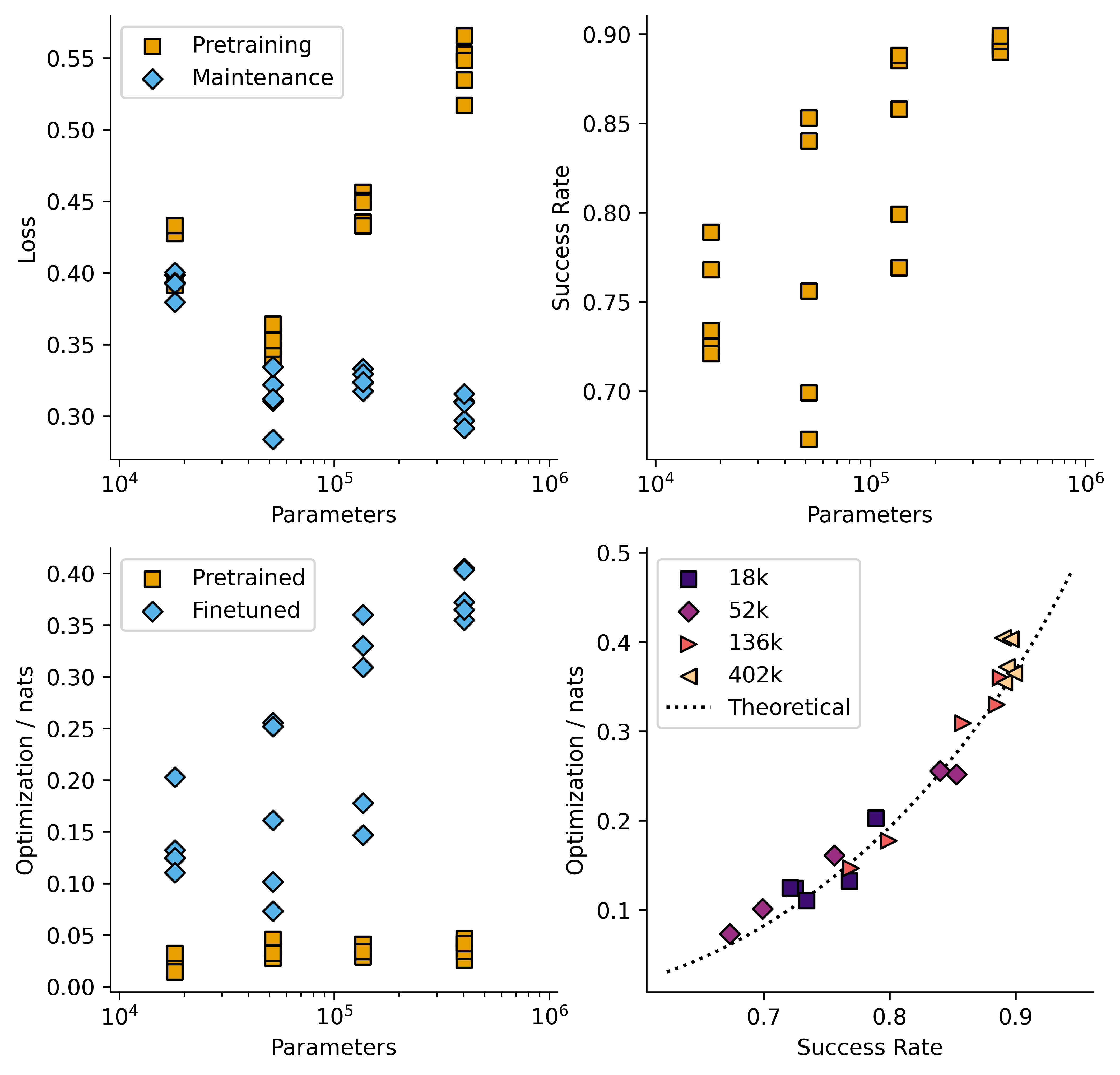
I then repeated the RL phase twice, once with $s_{t+1}\in \{0,4\}$ being reinforced,  ($n_{good}$ = 2) and once with $s_{t+1}\in \{0,1,2,4,5,6\}$ being reinforced ($n_{good}$ = 6). Here is a plot of success rate against model size across all three conditions.

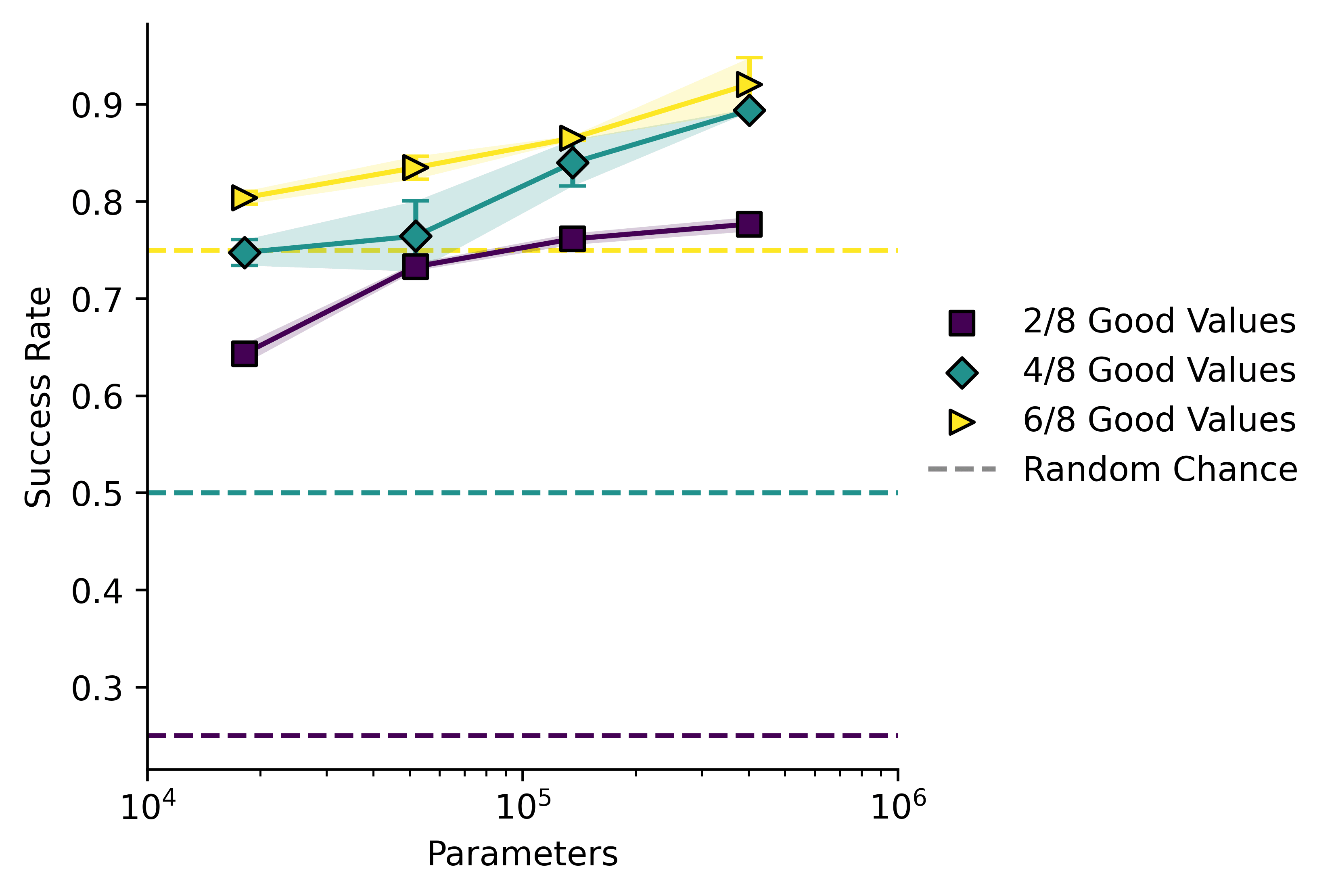
This plot shows mean $\pm$ standard error. In all cases model performance is a lot better than chance, and increases with model size.

Measuring Optimization

I used a Monte Carlo simulation to measure the nats of optimization that are being applied to $s_{t+1}$ using the split-history method I've previously outlined. This involves taking the difference in entropy between two distributions:

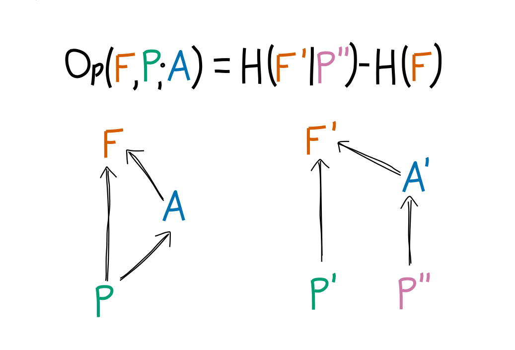
The algorithm in practice is this:

1. Take a bunch of sequence examples from the testing data, ensuring that $t$ is odd.
2. Feed them into the models to get a value for $s_t$, append to the sequence.
3. Use the sequence-generator to get a set of values for $s_{t+1}$
4. Look at the entropy of the resulting distribution over $s_{t+1}$, this is the optimized entropy.
5. For each sequence from the training data, and get a value of $s_t^{\prime }$ from this.
6. Repeat Steps 3-4 with the entire data set as $...,s_{t-2},s_{t-1}$ prepended to $s_t^{\prime }$, get one sample of "unoptimized" entropy
7. Repeat Steps 5-6 with each sequence from the initial dataset, take the average unoptimized entropy
8. Optimization = unoptimized entropy - optimized entropy

Here is a schematic illustration:

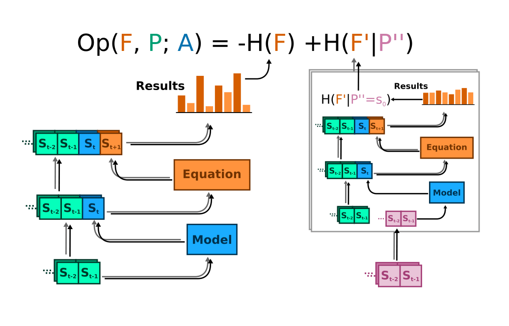
I ran this calculation 10 times with 200 sequences in $P$ and took an average to get an idea of the model's optimizing capability. I also tested the sequence-generating function's self-optimization.

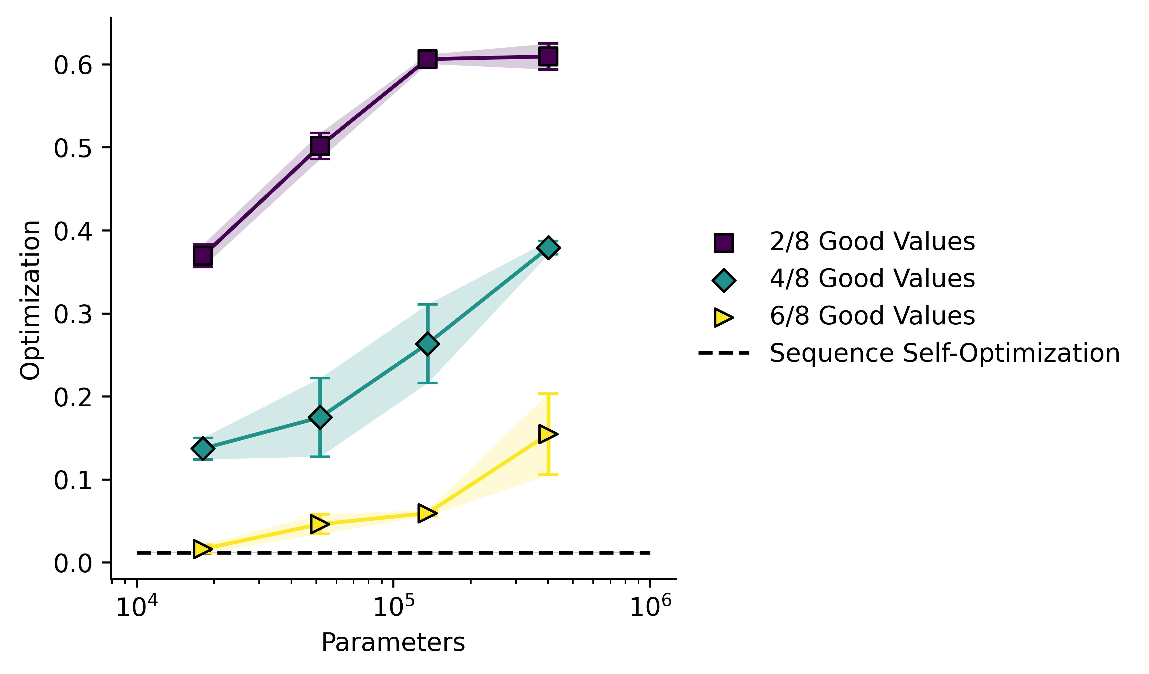
The fact that the sequence is optimizing itself mostly just amounts to saying that it is not a random walk, which we already knew. It is a good sanity check that all of the models get values either equal to or above this, and that optimization improves with model size.

Results

Optimization vs RL Success Rate

Optimization is calculated as the entropy difference of two distributions. Let us consider three parameters: $n$: the number of possible outcomes; $p$: the proportion of outcomes which are "successes"; and $s$:  the chance that the model achieves a successful outcome.

Assuming the model is "ambivalent" over successful outcomes, and likewise ambivalent over failed outcomes, then the value of $H\left(F\right)$ should be equal to $-s\ln \left(\frac{s}{np}\right)-(1-s)\ln \left(\frac{1-s}{n(1-p)}\right)$. If we then assume that all outcomes are equally likely when the model's outputs are "randomized", then $H\left(F^{\prime }|P^{\prime \prime }\right)$ is just $-\ln \left(\frac{1}{n}\right)$. If we take the difference we get the following expression:

$Op\approx s\ln \left(\frac{s}{np}\right)+(1-s)\ln \left(\frac{1-s}{n(1-p)}\right)-\ln \left(\frac{1}{n}\right)$

$Op\approx s\ln \frac{s}{p}+s\ln \frac{1}{n}+(1-s)\ln \frac{1-s}{1-p}+\ln \frac{1}{n}-s\ln \frac{1}{n}-\ln \frac{1}{n}$

$Op\approx s\ln \frac{s}{p}+(1-s)\ln \frac{1-s}{1-p}$

Now I can plot this theoretical value for $Op$ against $s$ for $p\in \{0.25,0.5,0.75\}$, and also plot all of the models on the same axes. Since we see a lot of run-to-run variation in model performance, I'll plot the raw data per model rather than statistics.

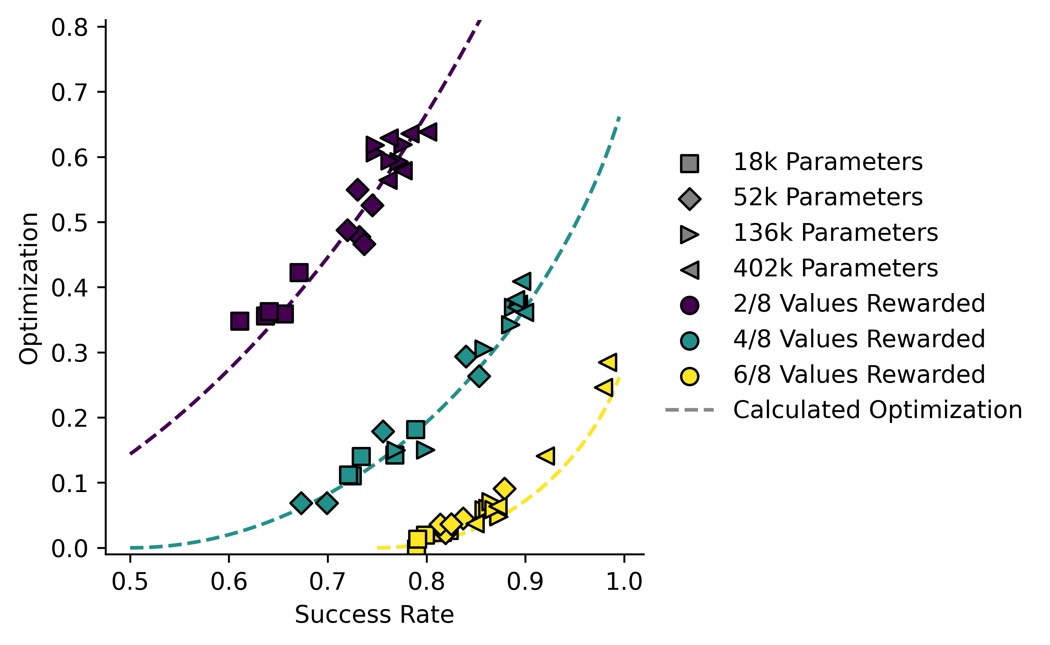
I tried to find some galaxy-brained variable change which would make those three curves the same, but I couldn't. Instead I will just plot the predicted value of $Op$ (based on their success rate) for each model against the actual value:

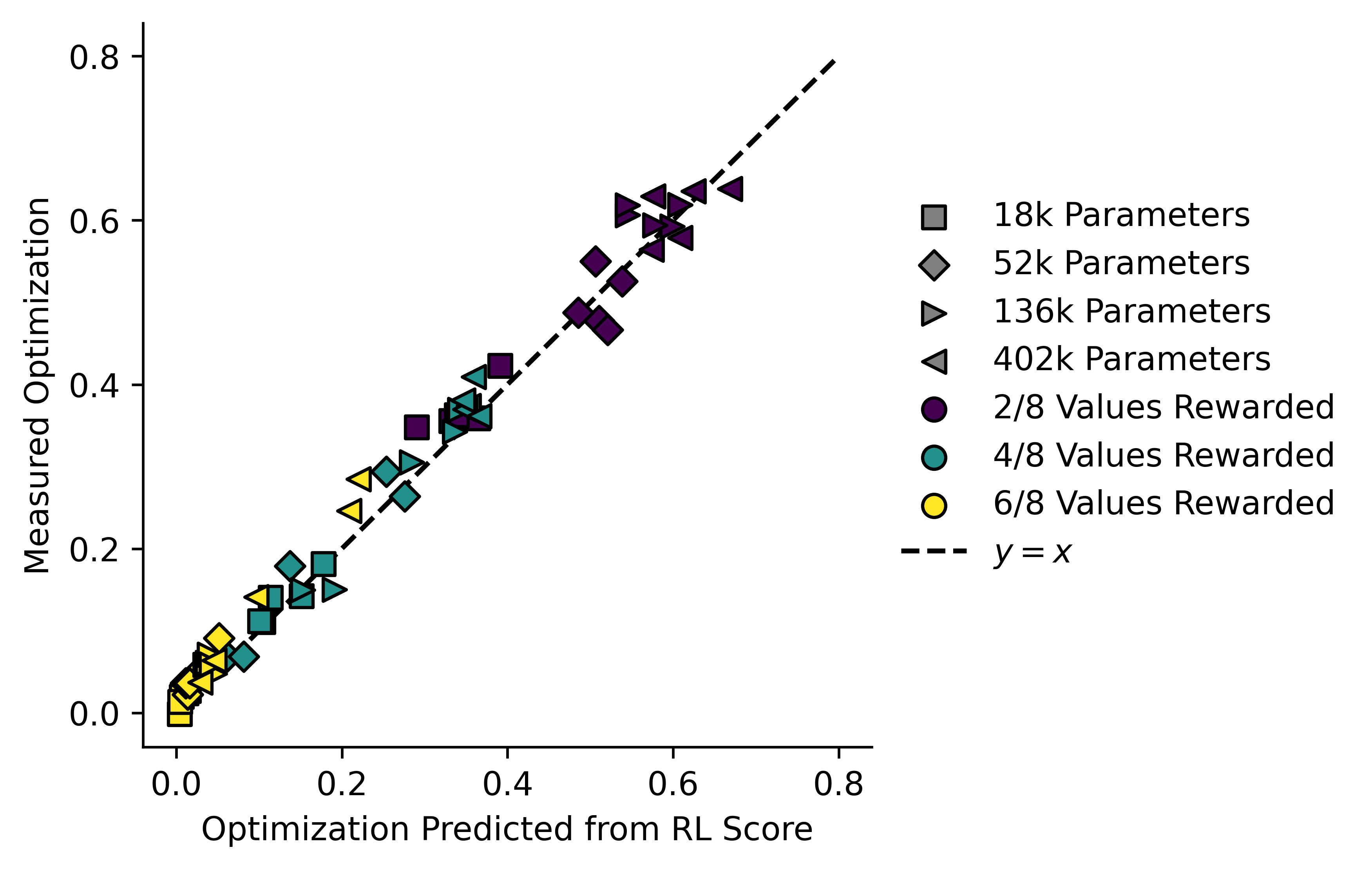
In theory none of the models should fall below the dashed line representing the equation derived above. In practice they do. Some of this is error in measurements, but I'm sure some of it is also due to errors in my assumptions. In particular the assumption that $H\left(F^{\prime }|P^{\prime \prime }\right)$ is completely flat is unlikely to hold.

On the other hand, there there is no reason at all why the models shouldn't fall quite far above the theoretical line. Consider the $n_{good}=6$ case, so successful values are$s_{t+1}\in \{0,1,2,4,5,6\}$. If the model ends up with a 85:15 ratio of values 2 and 3 for $s_{t+1}$(and never gets any other number, which is impossible in this specific case but that's not important for my point) then it will have a success rate of 0.85, which implies an $Op$ of 0.03, but its actual $Op$ will be 1.66!

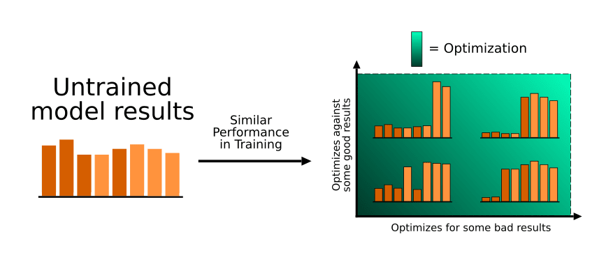
For a given training performance (in this case I've tried to make them all ~75% correct) the model might do one of several things:

1. Optimize for reinforced results and against non-reinforced results in an unbiased way
2. Optimize against non-reinforced results correctly, but only optimize for some of the successful results
3. Optimize for reinforced results correctly, but only optimize against some of the non-reinforced results
4. Behave in such a way that certain reinforced results are optimized against and certain non-reinforced results are optimized for.

The last three are examples of one type of inner misalignment. All three are characterized by excess optimization compared to the "correct" answer.

Cross-Objective Evaluation

The fact that most of the models don't sit far above the line shows that the RL is doing its job! They are (mostly) pursuing the training objective faithfully, without picking up on other objectives. I simulate what might happen if a model picks up on an "incorrect" objective by cross-evaluating models on each others' tasks:

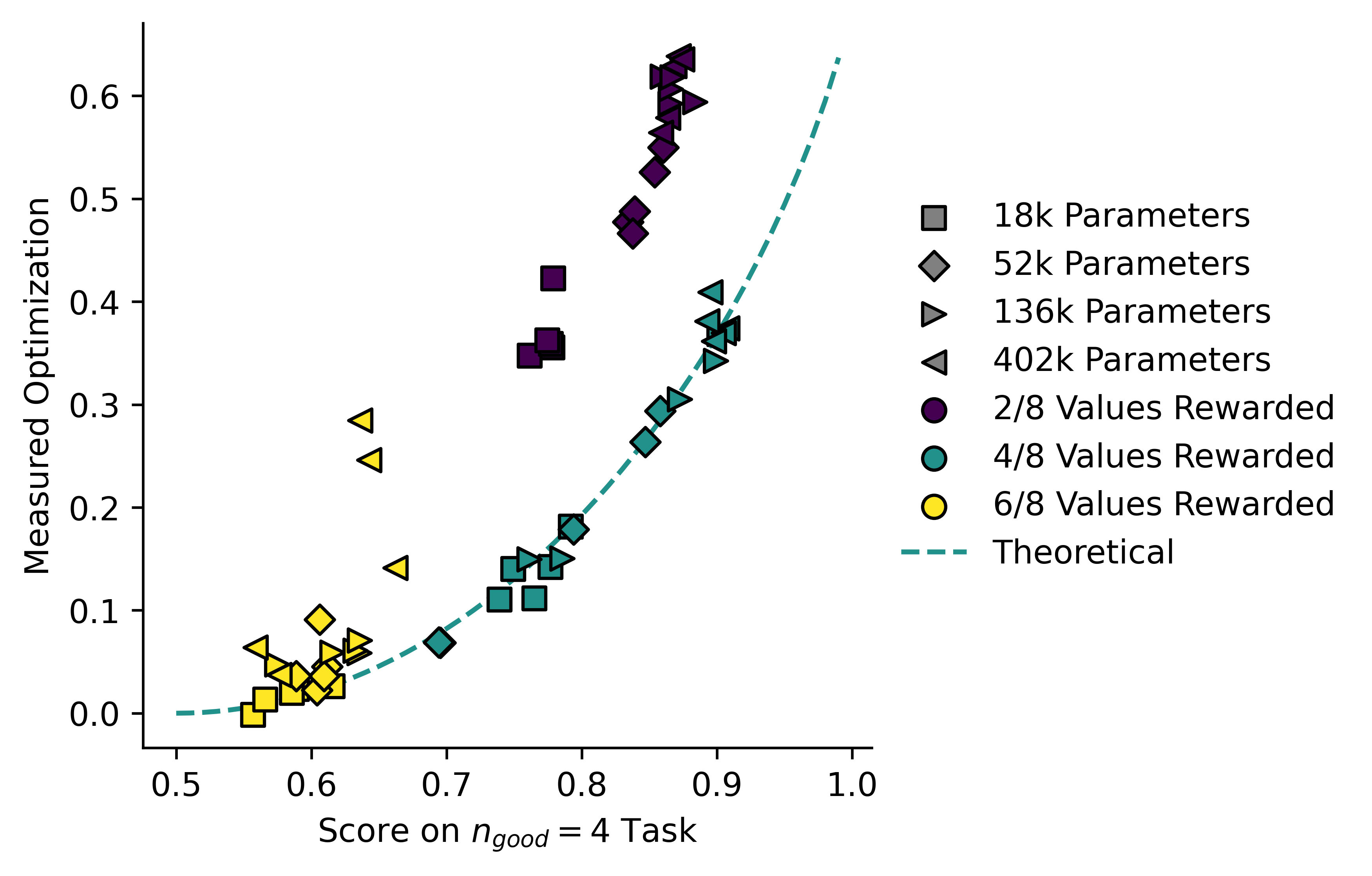
Now it becomes obvious that the $n_{good}=4$-trained models are behaving correctly whereas the other models are not. This is important since a model trained on the $n_{good}=2$ task will typically have a good score on the $n_{good}=4$ task, sometimes even higher than a similarly-sized model trained on the $n_{good}=4$ task (!) but this plot clearly shows us that something is going wrong.

It becomes even clearer if we instead take the value of $Op$ implied by the formula from above, and plot it against the actual value of $Op$. Here are the results for all three tasks:

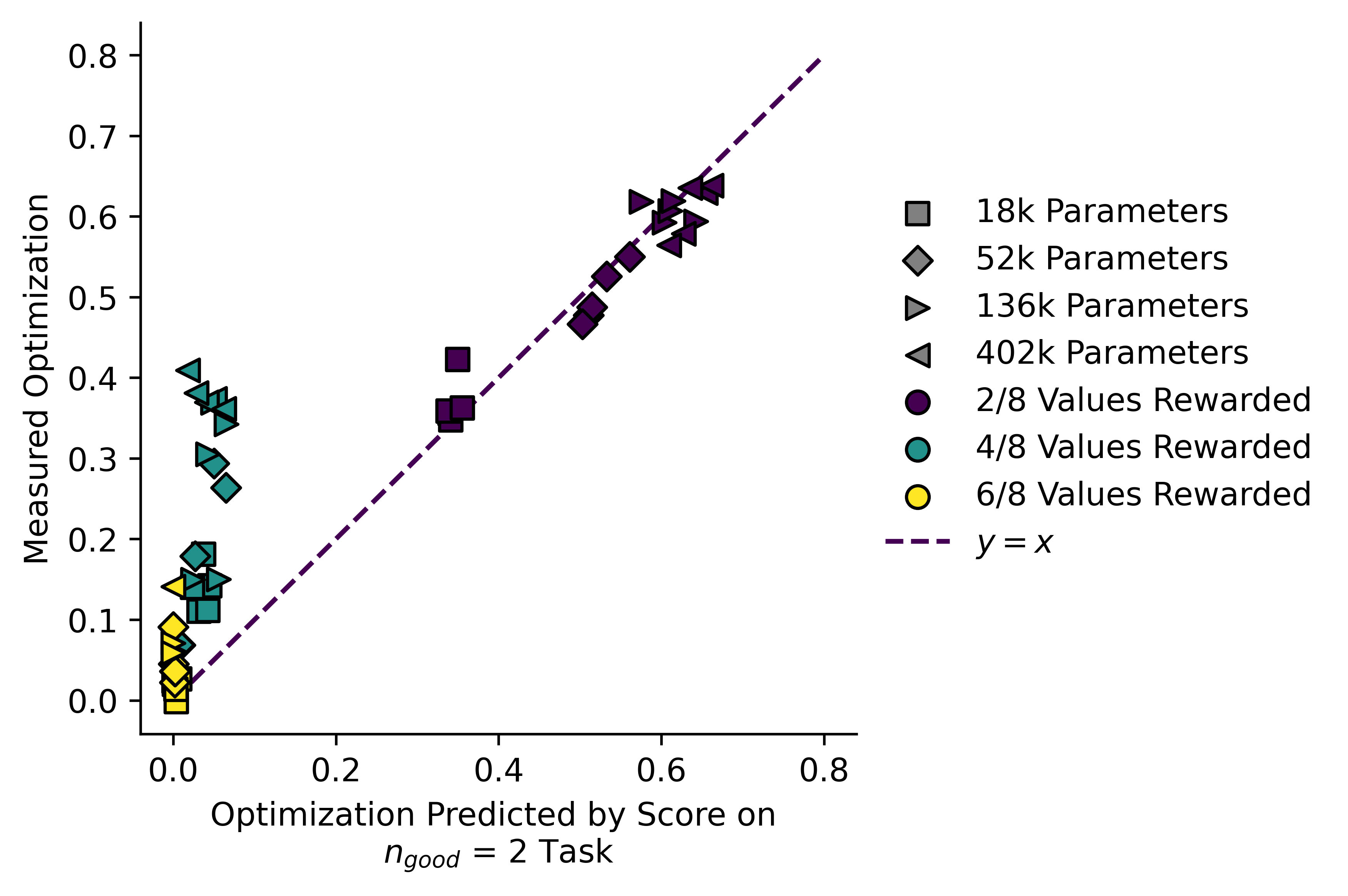
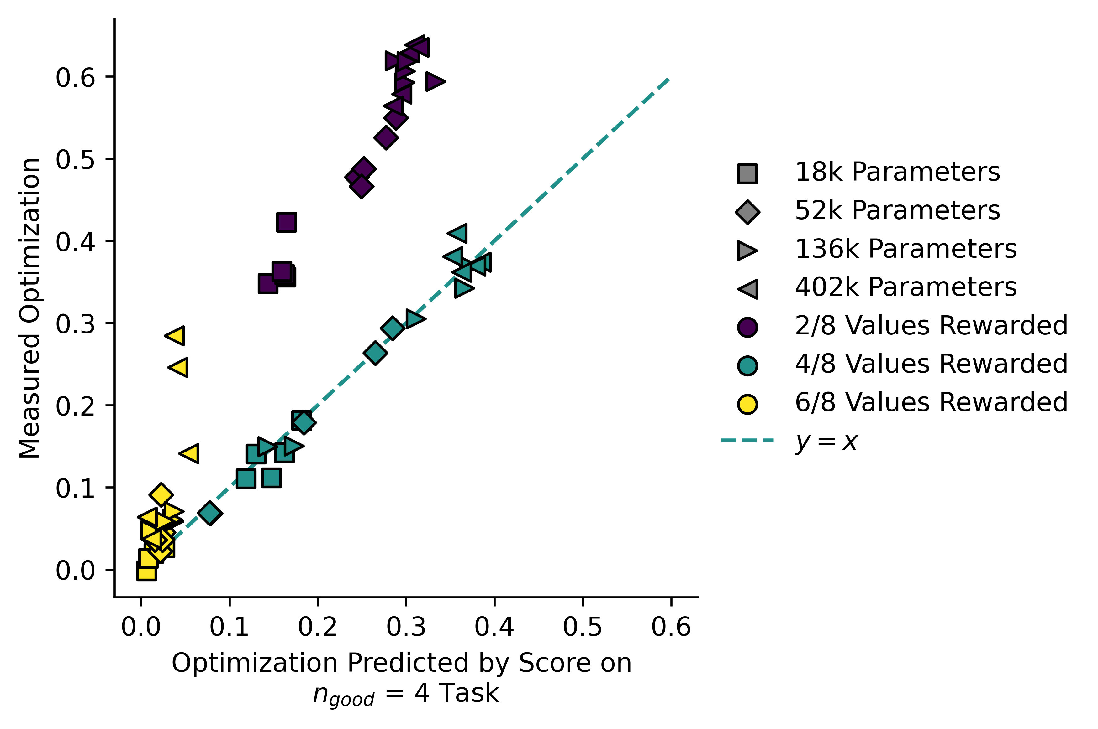
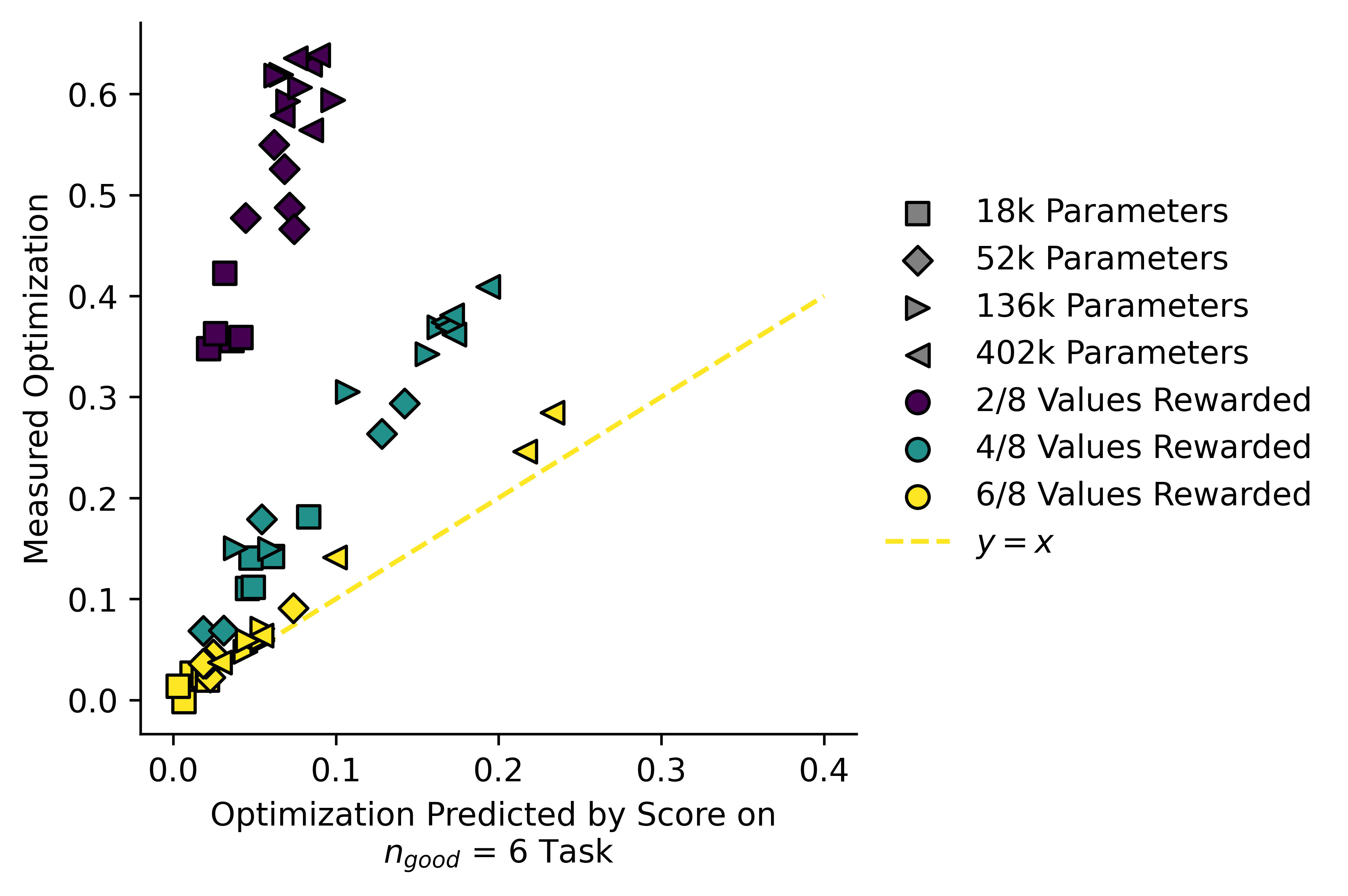
By comparing implied and measured $Op$, we can separate the models trained on a given reward signal from ones trained on a different reward signal, even when one of the reward signals is a subset of the other.

Optimization vs Impact

I will now take a second look at the measure for $Op$. What I really wanted all along is to measure a policy's impact on the world, and optimizing the future is only one way in which this can happen. Another way is flattening the possibilities out! Consider the following informal diagram. "Original" distribution is not well-defined here, the point is just to give an intuitive explanation:

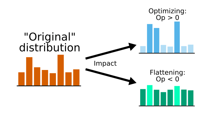
The motivation and derivations for this can be found in Appendix A, with longer proofs listed in Appendix B, but the upshot is that we can define a new function: $Imp(F,P;A)$ using the KL divergence of $F$ and $F^{\prime }$ like this:

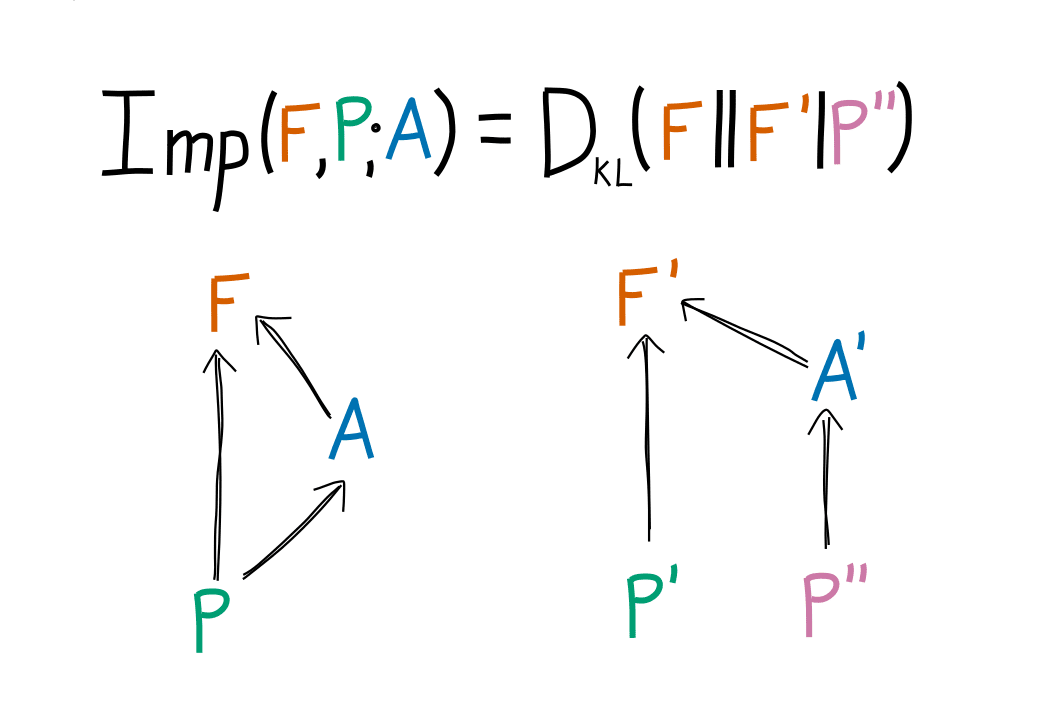
Which if we have a task success rate $s$ in $F$ and $s^{\prime }$ in $F^{\prime }$ must obey the following equation:

$Imp(F,P;A)\equiv D_{KL}(F\parallel F^{\prime }|P^{\prime \prime })\ge s\ln \frac{s}{s^{\prime }}+(1-s)\ln \frac{1-s}{1-s^{\prime }}\equiv {Imp}_{min}(F,P;A)$

This can be measured using the same split-history method used to measure $Op$:

The lower bound ${Imp}_{min}$ can be calculated from success rates and the two can be compared:

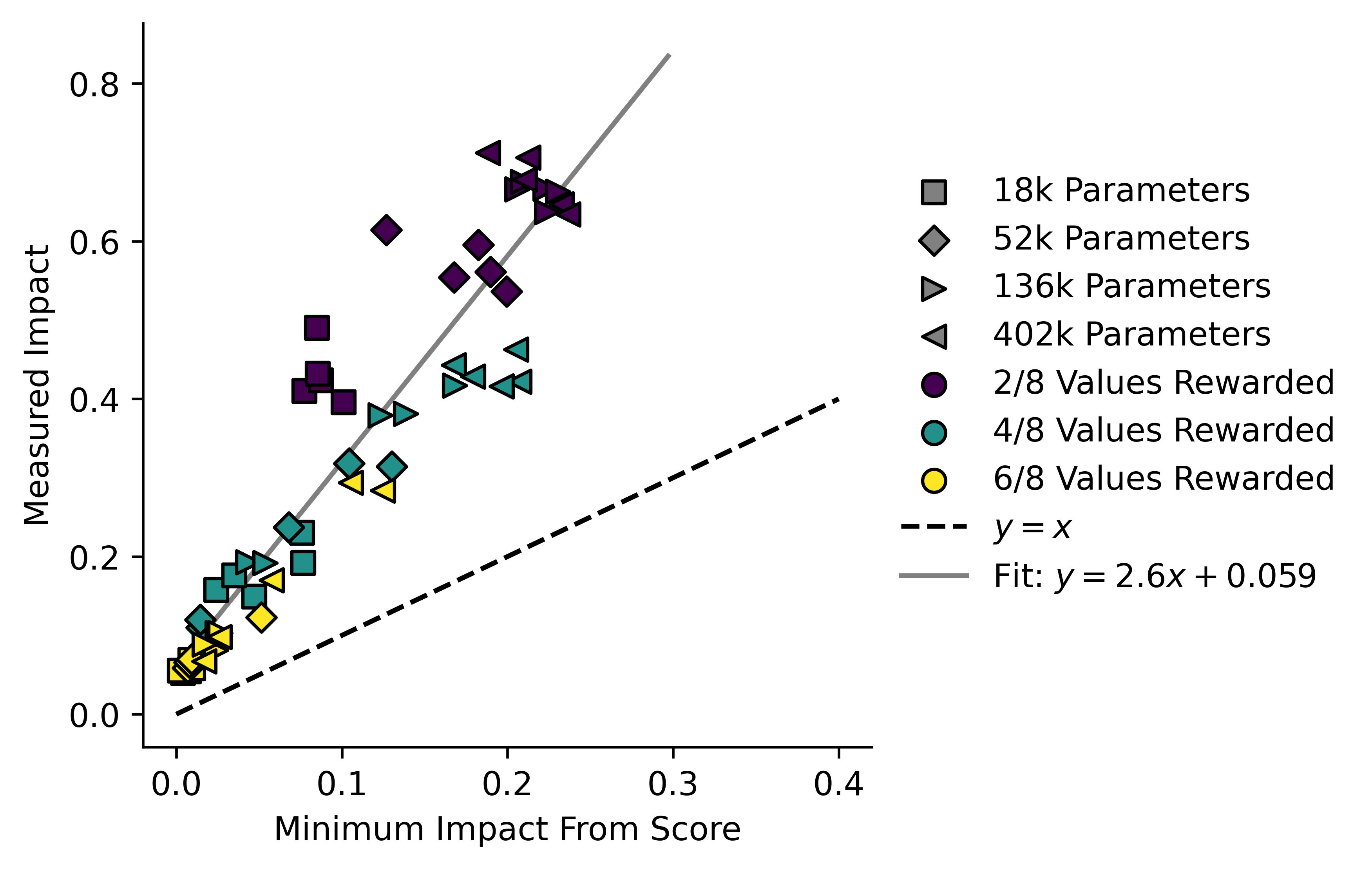
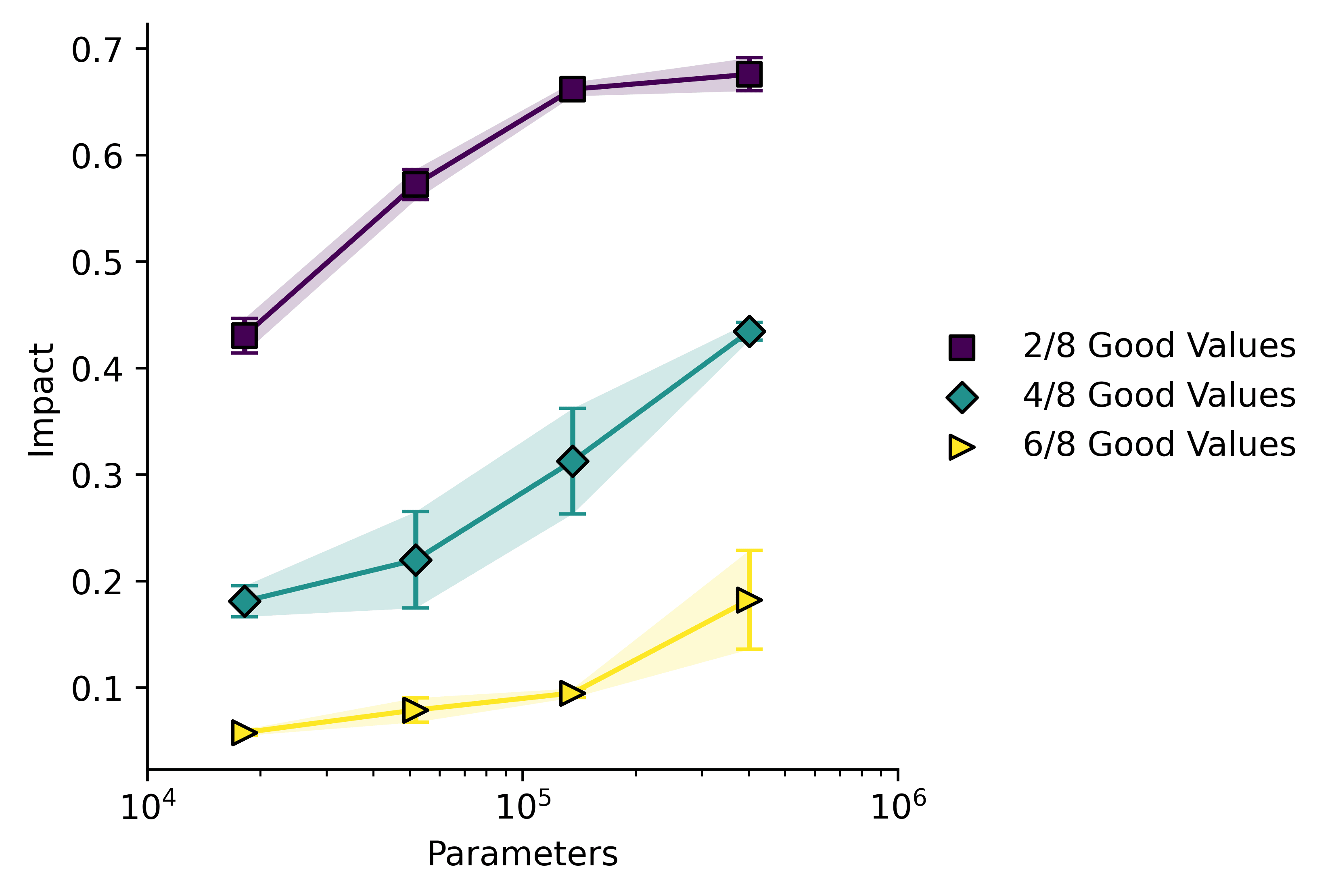
Larger models have a higher impact, but they also tend to have a lower ratio of $Imp/{Imp}_{min}$than do the smaller ones. The single-line fit is also somewhat misleading, and actually the models appear to lie on three separate lines. I note that the values of  ${Imp}_{min}$ are somewhat low in this case, rather than our measured impact being unexpectedly high. Our measure for $Imp$ may not be perfect in this case.

I think the difference between $Imp$ and ${Imp}_{min}$ tells us something. In this case it tells us that the success rates in $F^{\prime }$ are actually quite high:

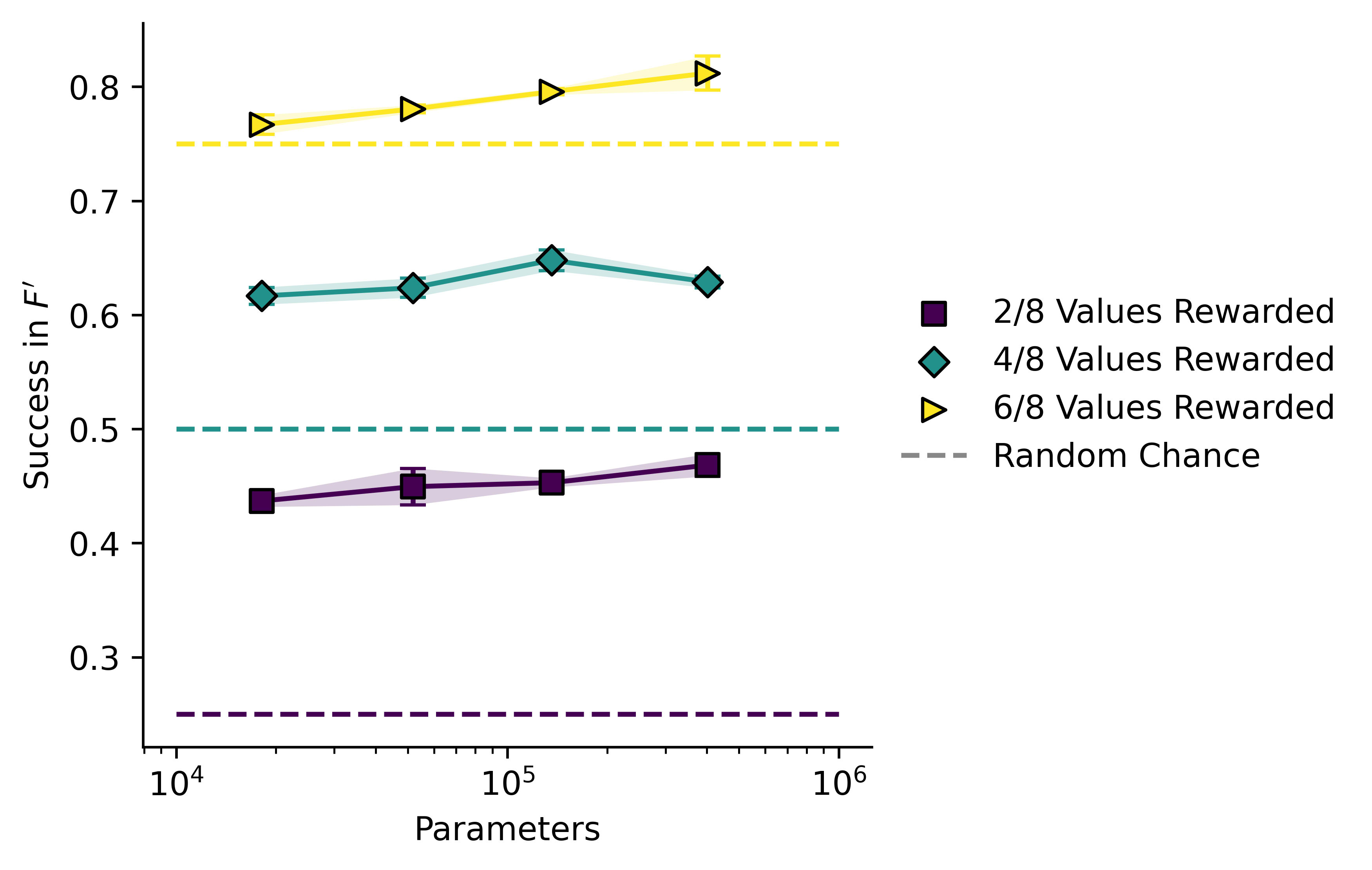
Success rate in $F^{\prime }$ doesn't scale very much at all with model size, which indicates that models of all sizes exhibit roughly the same bias in outputs, based on statistical regularities in the data (e.g. a "13" is more commonly followed by a "2" than a "15" is). It might also be an artefact stemming from an uneven distribution of numbers in our sequence by default.

This highlights an important point about split-history measures: they only pick up on the effects of "active" inference in the policy, not on biases in the outputs which are produced during training.  We don't have to use a split-history method to generate $F^{\prime }$, we can think up plenty of alternative ways to generate a comparison future, and therefore generate a family of measures for $Imp$ and $Op$:

• Use a privileged "Do nothing" token as the model's output
• Use a totally random output token
• Use an untrained model, or a pretrained (but not finetuned) model

Despite these problems, if we repeat cross-objective evaluation using $Imp$ we get these plots:

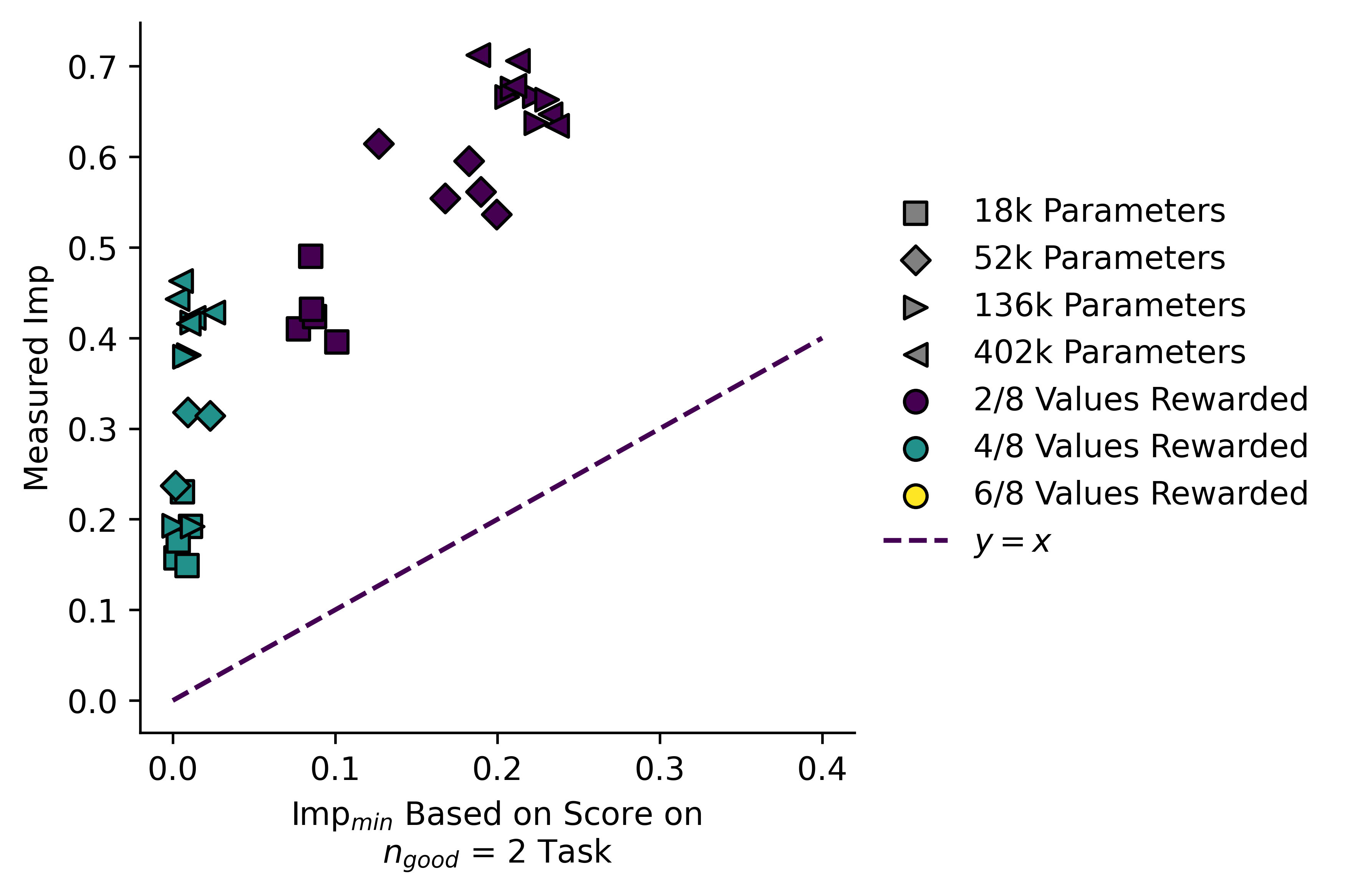
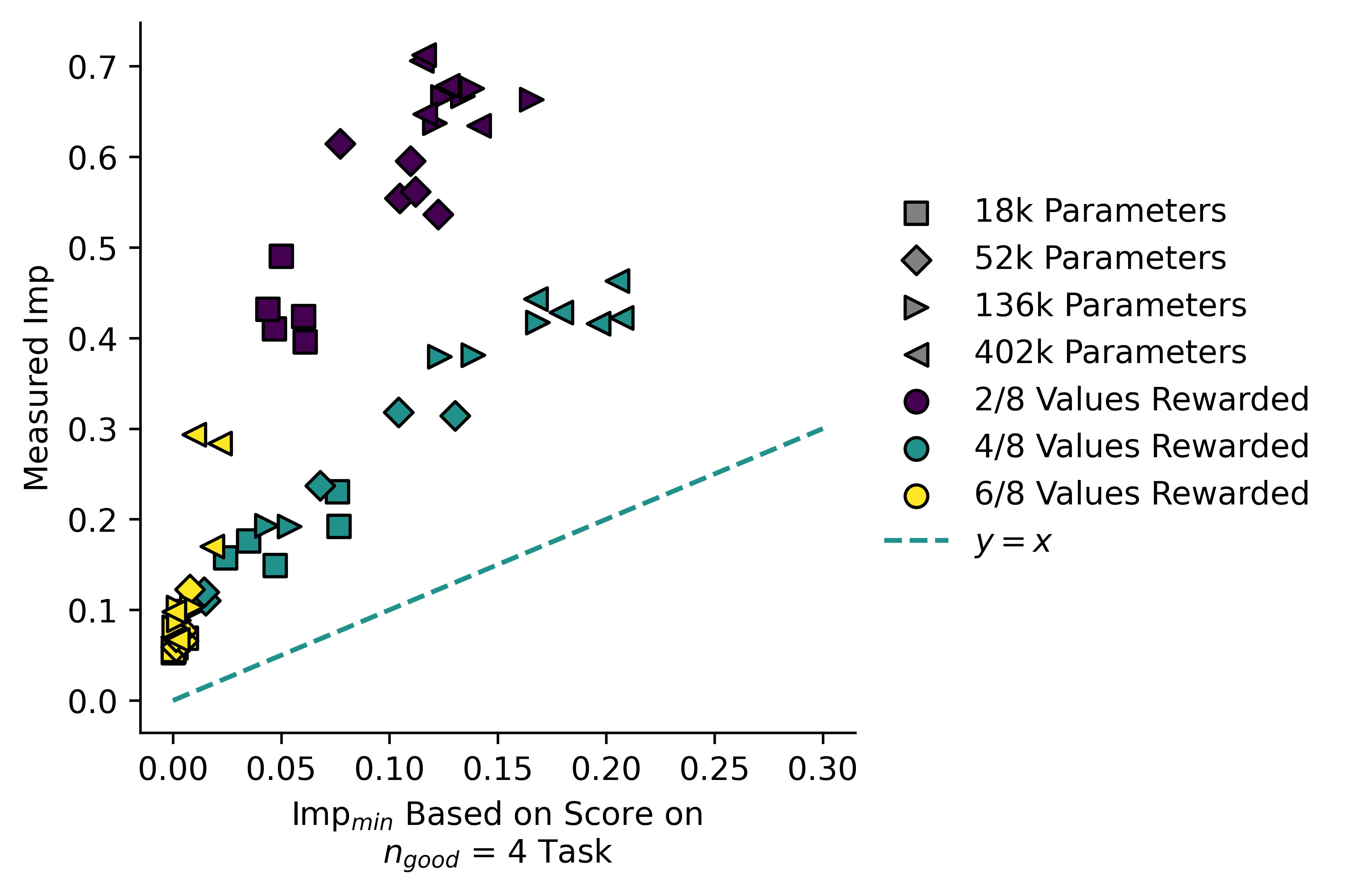
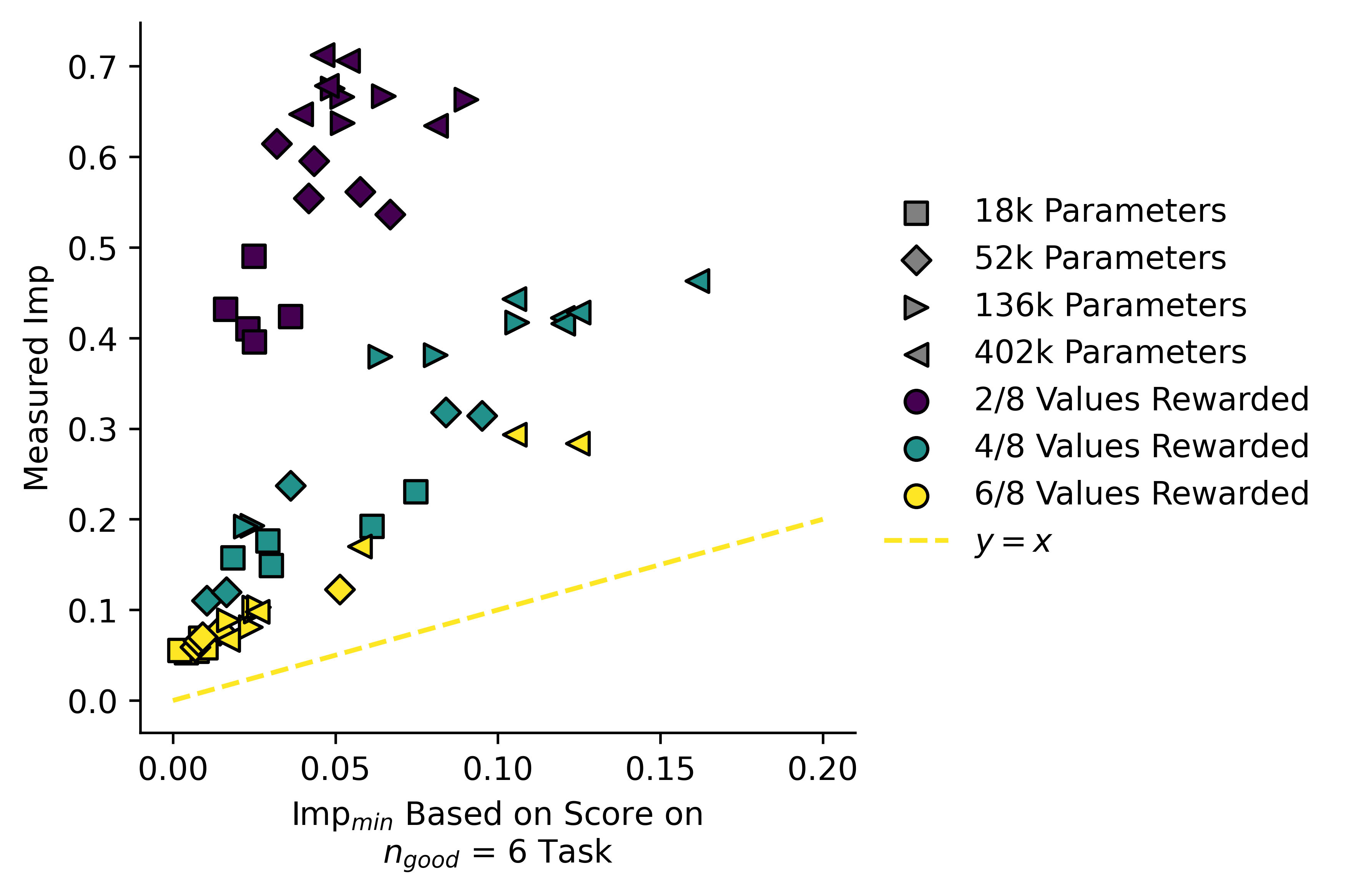
While the split is not as good as we saw with $Op$, it seems that models not trained on the "correct" fall along a line of lower gradient, and models trained on "incorrect" tasks have higher gradients i.e. the latter diverge from the ${Imp}_{min}$ line more rapidly.

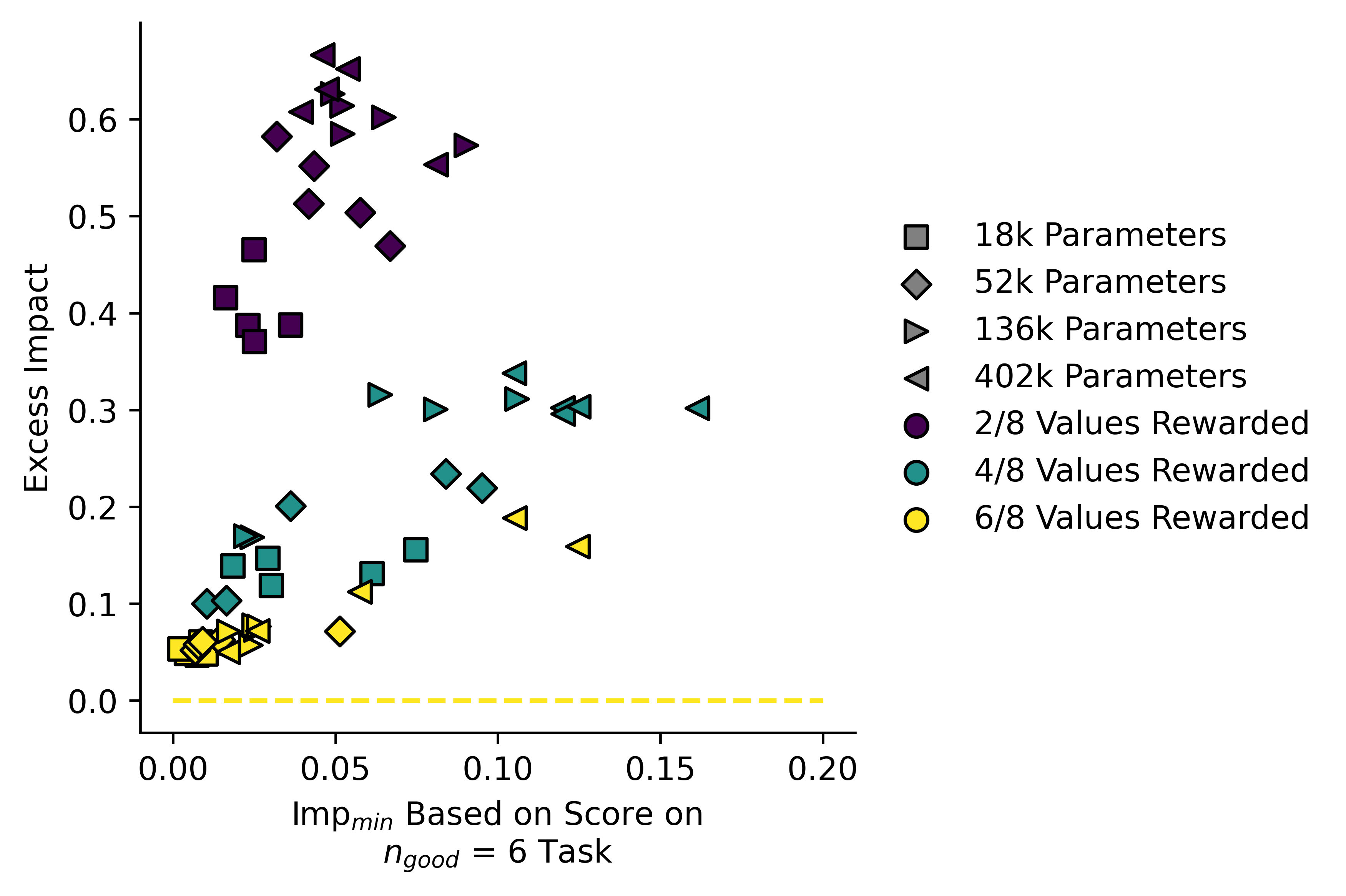
There are many potential ways to visualize what's going on here, two more of which are in Appendix C at the end of this post.

Model Self-Evaluation

A secondary goal of my work was to get models to evaluate their own optimizing power and impact. This is the reason for the maintenance training during finetuning. The self-evaluation scheme is the same as the optimization measuring scheme, except that instead of using the sequence-generating formula to get values for $s_{t+1}$, I used the model's own predictive power to get expected distributions over $s_{t+1}$ and $s_{t+1}^{\prime }$:

A plot showing measured optimization plotted against self-estimated optimzation. Models from the $n_{good}=6$ task tend to fall on the line $y=x$, but as $n_{good}$ decreases, models fall further above the line.

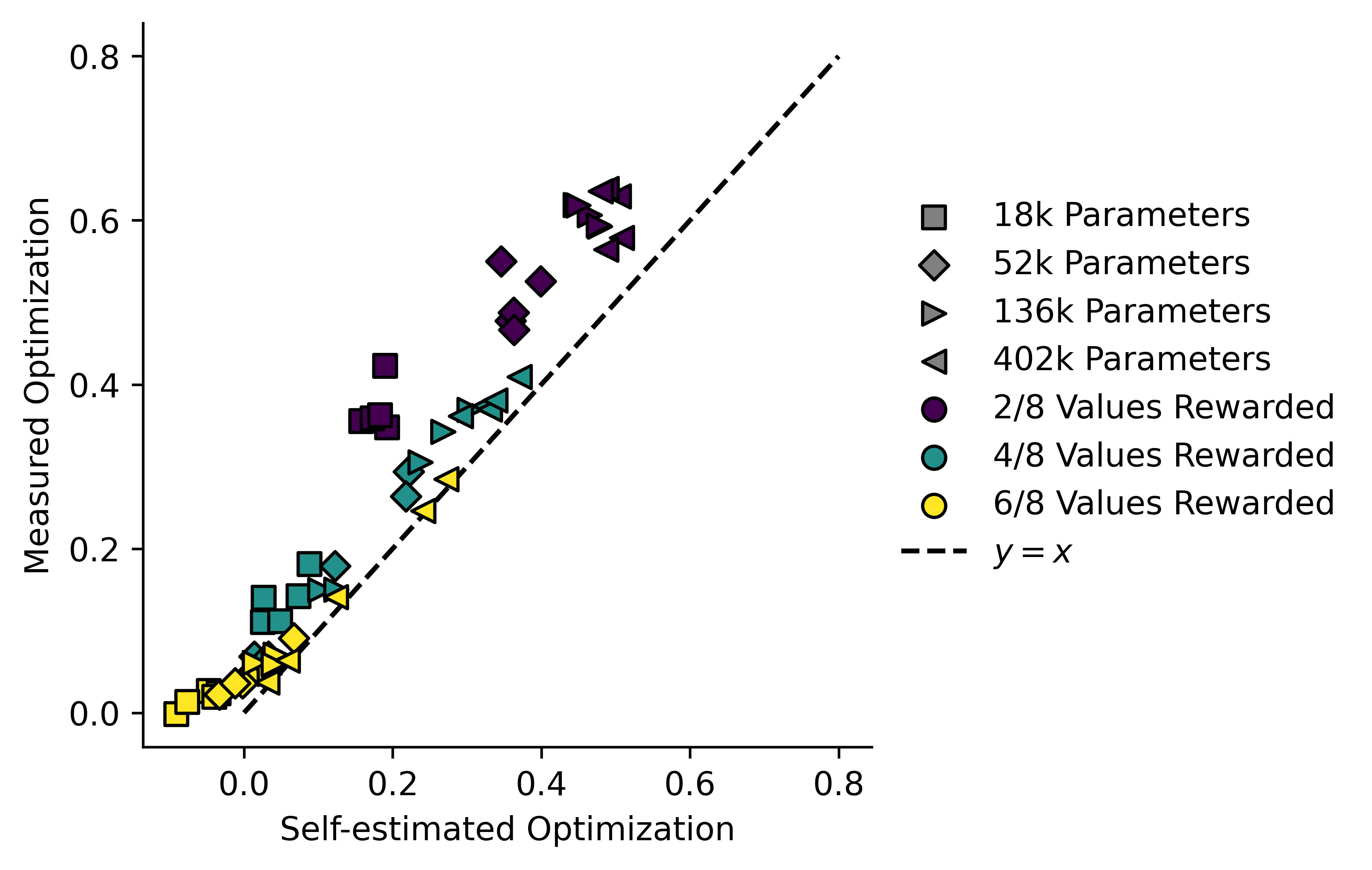
I suspect what's happened here is bog standard model bias. The more heavily the model is optimizing, the less even the distribution of examples of $s_{t+1}$ it gets fed during the maintenance training. This might make it more biased towards predicting the rewarded variables after any sequence, which would cause it to underestimate $Op$.

The same can be done for $Imp$:

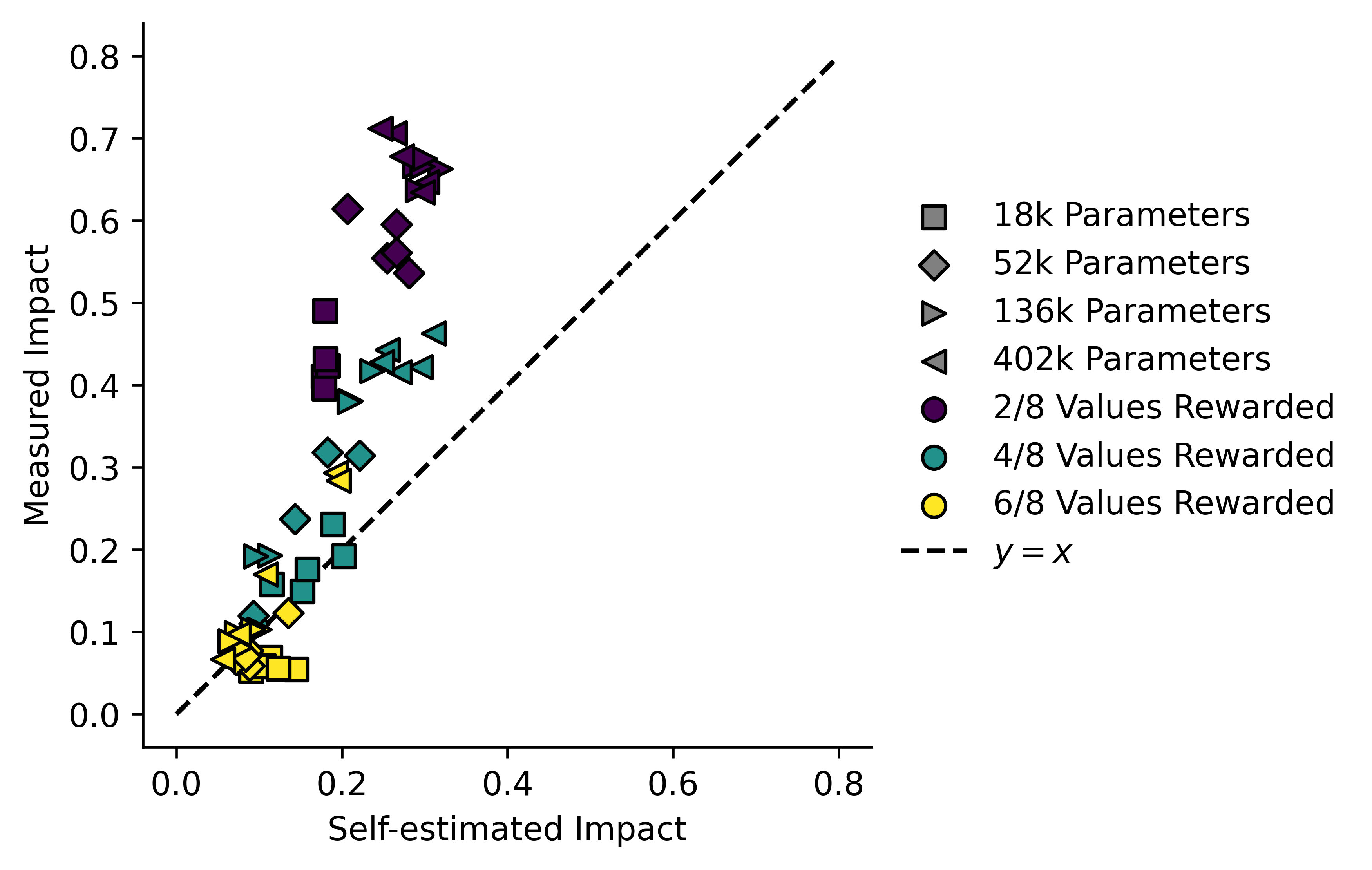
Which gives even worse results! I'm not sure whether or not this is also model bias. I don't have a tremendous amount of experience with ML, so I will not pursue this further in this post.

Conclusions

The measure I've introduced for $Op$ seems to be predicted very well by theory, and might have utility in detecting how well a policy's results line up with an RL task when it can be predicted accurately. The measure for $Imp$ has some issues but shows some success towards the same goal. These can be considered complementary measures in many ways:

Optimization	Impact
Can be positive or negative, the sign gives us information	Always $\ge 0$
Can be cancelled out by opposite-signed optimization elsewhere	Always a positive value, always at least adds up across different sources
No easy way to calculate theoretical values of Op in general (that I've found)	${Imp}_{min}$ can be calculated for any success/failure RL task
Excellent at identifying model behaviour in this case	Less good at identifying model behaviour in this case

I would be interested in applying both of these to more complex ML systems, but at the moment I don't any specific plans to do so, due to my very limited experience with ML. In Appendix A I also present equivalent measures which can be applied to the activations of a neural network.

A theoretical limitation of this work is that ${Imp}_{min}$ can only be calculated when a task is binary success/failure. If the policy is trying to maximize some function world-state then there's no simple formula for ${Imp}_{min}$ based on RL score. Work on these systems must either develop new maths or or find a way to break down utility maximization into a series of success/failure tasks, which can separately be evaluated for impact.

One practical limitation is in the self-evaluation stage. If the model's self-evaluation is biased, the measures of $Op$ and $Imp$ will be as well. This is especially problematic if $Op$ or $Imp$ is underestimated, allowing the policy to "lie" to us about how much optimization/impact it is doing. My wild guess is that AIs which include explicit world-modelling (such as DreamerV3) will be less biased by default, but that attempts at introducing impact regularization might reintroduce bias.

Alex Turner's Existing Work

The expression for impact that I present here is totally independent with the AUP measure of impact as proposed by Alex Turner in Towards a New Impact Measure [AF · GW]. There might be some subtle way in which they're related but I haven't thought about this enough to say more. I've also read World State is the Wrong Abstraction for Impact [LW · GW] and agree with some of the points presented.

In response I would say that the metric I present here relies strongly on a model $F$ of the future world state, so only details captured in $F$ can affect the impact. In the limit where the future states only consist of $f\in \{success,failure\}$, then impact is trivially equal to the lower bound and excess impact = 0.

Appendices

Appendix A: Impact and Differential Impact

Derivation of $Imp$

I present the motivation for, and derivation of, the measure of $Imp$ which I've used in this post. Returning to my estimator for $Op$:

$Op\approx s\ln \frac{s}{p}+(1-s)\ln \frac{1-s}{1-p}$

If we think these being two distributions over $\{success,failure\}$ and think of $p$ as the probability of succeeding by chance, this becomes the formula for a Kullback-Liebler divergence. For a quick recap, the KL divergence of two distributions over a variable $x\in \chi$ follows this formula:

$D_{KL}(P\parallel Q)=\sum _{x\in \chi }P\left(x\right)\ln \frac{P\left(x\right)}{Q\left(x\right)}$

We could also estimate the probability of succeeding by chance using the split-history method. Let $s$ be the success rate in $F$, and $s^{\prime }$ be the success rate in $F^{\prime }$:

$s\ln \frac{s}{s^{\prime }}+(1-s)\ln \frac{1-s}{1-s^{\prime }}$

I will now present some results about KL divergences. I will start by defining ${\chi }_s\subset \chi$ as the successful outcomes. Let us define a "baseline" probability distribution $P\left(x\right)$ and from it a "baseline" success rate $s_0$:

$s_0=\sum _{x_s\in {\chi }_s}P\left(x_s\right)$ 

Now imagine a policy acts on this distribution $P\left(x\right)$ and changes it to a new distribution. If this policy has a success rate $s\in [s_0,1]$, I define $Q\left(x\right)$ as follows:

 $Q\left(x\right)=\{\begin{array}{cc}\frac{s}{s_0}P\left(x\right)& x\in {\chi }_s\\ \frac{1-s}{1-s_0}P\left(x\right)& x\notin {\chi }_s\end{array}$

This is what we might expect to be the effects of a "minimum impact" policy: it makes successful outcomes more likely and unsuccesful outcomes less likely while leaving relative probabilities otherwise intact. The KL-divergence between $Q$ and $P$ can then be calculated, and it looks familiar:

$D_{KL}(Q\parallel P)=s\ln \frac{s}{s_0}+(1-s)\ln \frac{1-s}{1-s_0}$

This is the minimum KL divergence possible in shifting a distribution to achieve a given success rate. If we change the variable names to $Q\to F,P\to F^{\prime }|P^{\prime \prime },s_0\to s^{\prime }$ this allows us to write down the original relation for a policy's impact:

$Imp(F,P;A)\equiv D_{KL}(F\parallel F^{\prime }|P^{\prime \prime })\ge s\ln \frac{s}{s^{\prime }}+(1-s)\ln \frac{1-s}{1-s^{\prime }}\equiv {Imp}_{min}(F,P;A)$

Differential Impact

In this case "differential" means "to do with differentiation". I've studied a construct I call differential optimization in the past, as it pertains to functions of real-valued variables. In this case if we have the functions $A=f\left(P\right)$, $F=g(A,P)\equiv h\left(P\right)$ we can define the following value:

$C(F,P;A)=\frac{\partial F}{\partial P}{|}_{Avaries}/\frac{\partial F}{\partial P}{|}_{Aconstant}\equiv \frac{dh}{dP}/\frac{\partial g}{\partial P}$

Intuitively, if $A$ is "optimizing" $F$, then when it is allowed to vary, $C\le 1$ since $F$ will change less when we allow $A$ to change than when we fix $A$. This led to the derivation of the differential optimization $Op=-\ln \left(C\right)$.

This can be extended to a differential impact metric:

 $Imp\equiv -\ln \left(C\right)+C(C-1)$

This has a minimum $Imp=0$ at $C=1$, but it is speculative and has not been tested, so while I will present it here I can give no guarantees at all about its utility.

We can also extend this to vector-valued $P,F$. If we define $J_g$ as the Jacobian when $A$ varies, and $J_h$ as the Jacobian when $A$ is constant, then $C=J_g^{-1}{J}_h$ we get the following values for $Op$ and $Imp$:

$Op=-\ln |C|\equiv \ln |J_g|-\ln |J_h|$

$Imp=-\ln |C|+Tr\left(C{C}^T\right)-Tr\left(C\right)$

If $P$ and $F$ do not have the same dimension, then $J_g^{-1}$ does not exist and instead the following construction must be used:

$Op=\frac{1}{2}\ln |J_g{J}_g^T|-\frac{1}{2}\ln |J_h{J}_h^T|$

$Imp=\frac{1}{2}\ln |J_g{J}_g^T|-\frac{1}{2}\ln |J_h{J}_h^T|+Tr\left(J_h{J}_h^T\right(J_g{J}_g^T{)}^{-1})-Tr(J_g{J}_h^T\left(J_g{J}_g^T{)}^{-1}\right)$

The motivation for constructions like this is to apply them to the activations of neural networks. For a network with width $w$, and a backpropagation time of $t$, I believe the time-complexity of this contains a polynomial term in $w$ (possibly $O\left(w^5\right(\log w{)}^2)$ if using Bareiss algorithm) for the matrix inverse, and a term in $w\times t$.

Appendix B: Proofs

Derivation and proof of $Imp\ge {Imp}_{min}$

$D_{KL}(Q\parallel P)=\sum _{x_s\in {\chi }_s}\frac{s}{s_0}P\left(x_s\right)\ln \frac{\frac{s}{s_0}P\left(x_s\right)}{P\left(x_s\right)}+\sum _{x_u\notin {\chi }_s}\frac{1-s}{1-s_0}P\left(x_u\right)\ln \frac{\frac{1-s}{1-s_0}P\left(x_u\right)}{P\left(x_u\right)}$

$D_{KL}(Q\parallel P)=\frac{s}{s_0}\sum _{x_s\in {\chi }_s}P\left(x_s\right)\ln \frac{s}{s_0}+\frac{1-s}{1-s_0}\sum _{x_u\notin {\chi }_s}P\left(x_u\right)\ln \frac{1-s}{1-s_0}$

$D_{KL}\left(Q\right|P)=\frac{s}{s_0}\times s_0\ln \frac{s}{s_0}+\frac{1-s}{1-s_0}\times (1-s_0)\ln \frac{1-s}{1-s_0}$

$D_{KL}(Q\parallel P)=s\ln \frac{s}{s_0}+(1-s)\ln \frac{1-s}{1-s_0}$

I will prove that this choice of $Q$ is a global minimum of $D_{KL}(Q\parallel P)$ for a fixed $P$.

Consider a distribution $R=Q+\delta Q$, which involves moving some amount of probability mass $\delta$ from $x_1$ to $x_2$. Without loss of generality, take both to be in ${\chi }_s$ (they must both be in either ${\chi }_s$ or ${\chi }_s^C$ so that $R(x\in {\chi }_s)=s$ holds) Consider the value of

$D_{KL}(R\parallel P)-D_{KL}(Q\parallel P)$

Trivially we only need to look at the components relevant to $x_1$ and $x_2$:

$R\left(x_1\right)\ln \frac{R\left(x_1\right)}{P\left(x_1\right)}+R\left(x_2\right)\ln \frac{R\left(x_2\right)}{P\left(x_2\right)}-Q\left(x_1\right)\ln \frac{Q\left(x_1\right)}{P\left(x_1\right)}-Q\left(x_2\right)\ln \frac{Q\left(x_2\right)}{P\left(x_2\right)}$

Expand values of $R\left(x\right)$:

$\left(Q\right(x_1)-\delta )\ln \frac{\frac{s}{s_0}P\left(x_1\right)-\delta }{P\left(x_1\right)}+\left(Q\right(x_2)+\delta )\ln \frac{\frac{s}{s_0}P\left(x_2\right)+\delta }{P\left(x_2\right)}-Q\left(x_1\right)\ln \frac{\frac{s}{s_0}P\left(x_1\right)}{P\left(x_1\right)}-Q\left(x_2\right)\ln \frac{\frac{s}{s_0}P\left(x_2\right)}{P\left(x_2\right)}$

Expand and collect factors of $Q\left(x\right)$, cancelling the $P\left(x\right)$ on the bottom:

$Q\left(x_1\right)\ln \frac{\frac{s}{s_0}P\left(x_1\right)-\delta }{\frac{s}{s_0}P\left(x_1\right)}-\delta \ln \frac{\frac{s}{s_0}P\left(x_1\right)-\delta }{P\left(x_1\right)}+Q\left(x_2\right)\ln \frac{\frac{s}{s_0}P\left(x_2\right)+\delta }{\frac{s}{s_0}P\left(x_2\right)}+\delta \ln \frac{\frac{s}{s_0}P\left(x_2\right)+\delta }{P\left(x_2\right)}$

Collect the factors of $\delta$, expand stuff to a $\ln (1+y)$ form:

$Q\left(x_1\right)\ln (1-\frac{s_0}{s}\frac{\delta }{P\left(x_1\right)})+Q\left(x_2\right)\ln (1+\frac{s_0}{s}\frac{\delta }{P\left(x_2\right)})+\delta [\ln \frac{\frac{s}{s_0}P\left(x_2\right)+\delta }{P\left(x_2\right)}-\ln \frac{\frac{s}{s_0}P\left(x_1\right)-\delta }{P\left(x_1\right)}]$

$Q\left(x_1\right)\ln (1-\frac{s_0}{s}\frac{\delta }{P\left(x_1\right)})+Q\left(x_2\right)\ln (1+\frac{s_0}{s}\frac{\delta }{P\left(x_2\right)})+\delta [\ln (1+\frac{s_0}{s}\frac{\delta }{P\left(x_2\right)})-\ln (1-\frac{s_0}{s}\frac{\delta }{P\left(x_1\right)})]$

Use the taylor expansion $\ln (1+y)\approx y-\frac{1}{2}{y}^2...$ up to ${\delta }^2$.

$Q\left(x_1\right)(-\frac{s_0}{s}\frac{\delta }{P\left(x_1\right)}-\frac{1}{2}(-\frac{s_0}{s}\frac{\delta }{P\left(x_1\right)}{)}^2...)+Q(x_2\left)\right(\frac{s_0}{s}\frac{\delta }{P\left(x_2\right)}-\frac{1}{2}(\frac{s_0}{s}\frac{\delta }{P\left(x_2\right)}{)}^2...)+\delta [(\frac{s_0}{s}\frac{\delta }{P\left(x_2\right)}...)-(\frac{s_0}{s}\frac{\delta }{P\left(x_1\right)}...)]$

Sub in $Q\left(x\right)=\frac{s}{s_0}P\left(x\right)$, expand, cancel:

$-\frac{1}{2}{\delta }^2\frac{s_0}{s}(\frac{1}{P\left(x_1\right)}+\frac{1}{P\left(x_2\right)})+{\delta }^2\frac{s_0}{s}(\frac{1}{P\left(x_2\right)}+\frac{1}{P\left(x_1\right)})$

Subtract:

$\frac{1}{2}{\delta }^2\frac{s_0}{s}(\frac{1}{P\left(x_1\right)}+\frac{1}{P\left(x_2\right)})\ge 0$

Therefore $Q\left(x\right)$ is a local minimum of $D_{KL}(Q\parallel P)$ subject to our condition that $Q(X\in {\chi }_x)=s$. $D_{KL}(Q\parallel P)$ is convex in $Q$ for fixed $P$, therefore we have found the unique global minimum.

Derivation of Differential Impact

The measure of $Op$ based on entropy that I've used here was based on the following comparison to differential optimization:

Consider the network $A=P$, $F=P-(1-k)A$. This gives $C(F,P;A)=k$ and $Op(F,P;A)=-\ln k$.

This can be extended to an entropic measure of $Op$ by considering uncertainty over $P$, specifically:

 $P\sim N({\mu }_P,{\sigma }_P)$

$A\sim N({\mu }_P,{\sigma }_P)$

$F\sim N(k{\mu }_P,k{\sigma }_P)$

Using split-histories we get:

$P^{\prime },P^{\prime \prime }\sim N({\mu }_P,{\sigma }_P)$

$A^{\prime }\sim N({\mu }_P,{\sigma }_P)$

$F^{\prime }|P^{\prime \prime }=p^{\prime \prime }\sim N({\mu }_P-(1-k)p^{\prime \prime },{\sigma }_P)$

If we take $Op(F,P;A)=H\left(F^{\prime }|P^{\prime \prime }\right)-H\left(F\right)$ this gives the familiar value of $\ln k$. We may instead investigate the value of $Imp(F,P;A)=D_{KL}(F\parallel F^{\prime }|P^{\prime \prime })$. Letting $F\sim N({\mu }_1,{\sigma }_1)$, $F^{\prime }|P^{\prime \prime }\sim N({\mu }_2,{\sigma }_2)$ for brevity:

$Imp=\ln \left(\frac{{\sigma }_2}{{\sigma }_1}\right)+\frac{1}{2}\frac{{\sigma }_1^2+({\mu }_1,{\mu }_2{)}^2}{{\sigma }_2^2}-\frac{1}{2}$

Substituting:

${\mu }_1-{\mu }_2=k{\mu }_P-{\mu }_P+(1-k)p^{\prime \prime }=(1-k)p^{\prime \prime }-(1-k){\mu }_P$

$({\mu }_1-{\mu }_2{)}^2=(1-k{)}^2({\mu }_P^2-2{\mu }_P{p}^{\prime \prime }+p^{\prime \prime 2})$

Taking $E\left(\right({\mu }_1-{\mu }_2{)}^2)$ with respect to $p^{\prime \prime }$ requires taking $E\left(p^{\prime \prime }\right)={\mu }_P$, $E\left(p^{\prime \prime 2}\right)={\mu }_P^2+{\sigma }_P^2$:

$({\mu }_1-{\mu }_2{)}^2=(1-k{)}^2({\mu }_P^2-2{\mu }_P^2+{\mu }_P^2+{\sigma }_P^2)={\sigma }_P^2$

${\sigma }_1=k{\sigma }_P$

${\sigma }_2={\sigma }_P$

Substituting into our original equation:

$Imp=\ln \left(1/k\right)+\frac{1}{2}[k^2+(1-k{)}^2\frac{{\sigma }_P^2}{{\sigma }_P^2}]-\frac{1}{2}$

$Imp=-\ln \left(k\right)+\frac{1}{2}[k^2+1-2k+k^2]-\frac{1}{2}$

$Imp=-\ln \left(k\right)+k^2-k$

$Imp=-\ln \left(k\right)+k(k-1)$

Which, if we extend to $C$, gives

$Imp=-\ln \left(C\right)+C(C-1)$

Derivation of Multivariate Differential Impact and Optimization

Let us take vectors $p,a,f$, and $p^{\prime },p^{\prime \prime },a^{\prime },f^{\prime }$ in the same manner as above. Assume around some value of $p$ we have the following Jacobians.

$J_f=\frac{da}{dp}$ $J_g=\frac{\partial f}{\partial p}$  $J_h=\frac{df}{dp}$

Without loss of generality, take the means of all of these variables to be $0$. There exists a formula for transforming a multivariate normal distribution^[1].

$P\sim N(0,{\Sigma }_p)$

$A\sim N(0,J_f{\Sigma }_p{J}_f^T)$

$F\sim N(0,J_h{\Sigma }_p{J}_h^T)$

Now for $f^{\prime }|p^{\prime \prime }$, the mean will no longer be zero:

$F^{\prime }|P^{\prime \prime }=p^{\prime \prime }\sim N\left(\right(J_h-J_g)p^{\prime \prime },J_g{\Sigma }_p{J}_g^T)$

We can calculate the KL divergence of $D_{KL}(F\parallel F^{\prime }|P^{\prime \prime })$ using another formula^[2]: 

$\frac{1}{2}[\ln \frac{|{\Sigma }_2|}{|{\Sigma }_1|}-n_{dim}+Tr\left({\Sigma }_2^{-1}{\Sigma }_1\right)+({\mu }_2-{\mu }_1{)}^T{\Sigma }_2^{-1}({\mu }_2-{\mu }_1\left)\right]$

${\Sigma }_1=J_h{\Sigma }_p{J}_h^T$
${\Sigma }_2=J_g{\Sigma }_p{J}_g^T$
${\mu }_2-{\mu }_1=(J_h-J_g)p^{\prime \prime }$

Therefore our impact will be:

$\frac{1}{2}[\ln \frac{|J_g{\Sigma }_p{J}_g^T|}{|J_h{\Sigma }_p{J}_h^T|}-n_{dim}+Tr\left(\right(J_g{\Sigma }_p{J}_g^T{)}^{-1}{J}_h{\Sigma }_p{J}_h^T)+p^{\prime \prime T}(J_h-J_g{)}^T\left(J_g{\Sigma }_p{J}_g^T{)}^{-1}\right(J_h-J_g)p^{\prime \prime }]$

Taking the expected value of the third component is actually easy if you have access to the internet. We can see that it is of the form $E\left(v^{T}Mv\right)$ where $v$ is multivariate normal. This has a closed-form solution^[3]:

${\mu }^{T}M\mu +Tr\left(M\Sigma \right)$

Therefore we have the following expression:

$\frac{1}{2}[\ln \frac{|J_g{\Sigma }_p{J}_g^T|}{|J_h{\Sigma }_p{J}_h^T|}-n_{dim}+Tr\left(\right(J_g{\Sigma }_p{J}_g^T{)}^{-1}{J}_h{\Sigma }_p{J}_h^T)+Tr((J_h-J_g{)}^T\left(J_g{\Sigma }_p{J}_g^T{)}^{-1}\right(J_h-J_g){\Sigma }_p)]$

We can make some progress towards simplifying this if we take ${\Sigma }_p={\sigma }_{p}I$, which in this case lets us cancel everything out involving a ${\Sigma }_p$, since the scalar value of ${\sigma }_p$ commutes with all matrices, $|{\sigma }_{p}I|={\sigma }_p^{n_{dim}}$, and $({\sigma }_{p}I{)}^{-1}={\sigma }_p^{-1}I$. We will also assume that all the Jacobians are invertible.

$\frac{1}{2}[\ln \frac{|J_g{J}_g^T|}{|J_h{J}_h^T|}-n_{dim}+Tr\left(\right(J_g{J}_g^T{)}^{-1}{J}_h{J}_h^T)+Tr((J_h-J_g{)}^T\left(J_g{J}_g^T{)}^{-1}\right(J_h-J_g))]$

$\frac{1}{2}[\ln \frac{|J_g{J}_g^T|}{|J_h{J}_h^T|}-n_{dim}+Tr\left(\right(J_g{J}_g^T{)}^{-1}{J}_h{J}_h^T)+Tr(J_h^T\left(J_g^T{)}^{-1}{J}_g^{-1}{J}_h\right)-Tr\left(J_h^T\right(J_g^T{)}^{-1}{J}_g^{-1}{J}_g)-Tr(J_g^T\left(J_g^T{)}^{-1}{J}_g^{-1}{J}_h\right)+Tr\left(J_g^T\right(J_g^T{)}^{-1}{J}_g^{-1}{J}_g)]$

$\frac{1}{2}[\ln \frac{|J_g{J}_g^T|}{|J_h{J}_h^T|}-n_{dim}+Tr\left(\right(J_g{J}_g^T{)}^{-1}{J}_h{J}_h^T)+Tr(J_h^T\left(J_g{J}_g^T{)}^{-1}{J}_h\right)-Tr\left(J_h^T\right(J_g^T{)}^{-1})-Tr(J_g^{-1}{J}_h)+Tr(I)]$

$\frac{1}{2}[\ln \frac{|J_g{J}_g^T|}{|J_h{J}_h^T|}+Tr\left(\right(J_g{J}_g^T{)}^{-1}{J}_h{J}_h^T)+Tr(J_h^T\left(J_g{J}_g^T{)}^{-1}{J}_h\right)-Tr\left(J_h^T\right(J_g^T{)}^{-1})-Tr(J_g^{-1}{J}_h)]$

$\frac{1}{2}[\ln \frac{|J_g{J}_g^T|}{|J_h{J}_h^T|}+Tr\left(\right(J_g{J}_g^T{)}^{-1}{J}_h{J}_h^T)+Tr(J_h^T\left(J_g{J}_g^T{)}^{-1}{J}_h\right)-2Tr\left(J_g^{-1}{J}_h\right)]$

Using the cyclic property of the trace:

$\frac{1}{2}[\ln \frac{|J_g{J}_g^T|}{|J_h{J}_h^T|}+2Tr\left(\right(J_g{J}_g^T{)}^{-1}{J}_h{J}_h^T)-2Tr(J_g^{-1}{J}_h)]$

$\frac{1}{2}\ln \frac{|J_g{J}_g^T|}{|J_h{J}_h^T|}+Tr\left(\right(J_g^T{)}^{-1}{J}_g^{-1}{J}_h{J}_h^T)-Tr(J_g^{-1}{J}_h)$

$\frac{1}{2}\ln \frac{|J_g{J}_g^T|}{|J_h{J}_h^T|}+Tr\left(J_g^{-1}{J}_h{J}_h^T\right(J_g^T{)}^{-1})+Tr(J_g^{-1}{J}_h)$

$\frac{1}{2}\ln |J_g{J}_g^T(J_h{J}_h^T{)}^{-1}|+Tr(J_g^{-1}{J}_h\left(J_g^{-1}{J}_h{)}^T\right)-Tr\left(J_g^{-1}{J}_h\right)$

And if we define $C=J_g^{-1}{J}_h$ we get:

$-\ln |C|+Tr\left(C{C}^T\right)-Tr\left(C\right)$

This seems to have the form of $-\ln \left(C^2\right)+C^2-C$, and in fact if we consider $P$, $A$, and $F$ to just be concatenations of variables, which maeans all the $J$ matrices are diagonal, we see that our equation has the form.

$-\ln (\prod C)+\sum C^2-\sum C=\sum (-\ln C+C^2-C)$

Which is a nice sanity check. The value of $Op$ is just the entropy difference $\frac{1}{2}\ln {\Sigma }_2-\frac{1}{2}\ln {\Sigma }_1$ which simplifies to $-\ln |C|$ for free.

If the Jacobians are not invertible, but we assume that $J_g{J}_g^T$ is invertible, we instead get:

$Imp=\frac{1}{2}\ln |J_g{J}_g^T|-\frac{1}{2}\ln |J_h{J}_h^T|+Tr\left(J_h{J}_h^T\right(J_g{J}_g^T{)}^{-1})-Tr(J_g{J}_h^T\left(J_g{J}_g^T{)}^{-1}\right)$

Appendix C: Supplementary Plots

Other Ways to Visualize Impact Plots

Here I plotted the "Impact ratio" $Imp/{Imp}_{min}$ against ${Imp}_{min}$:

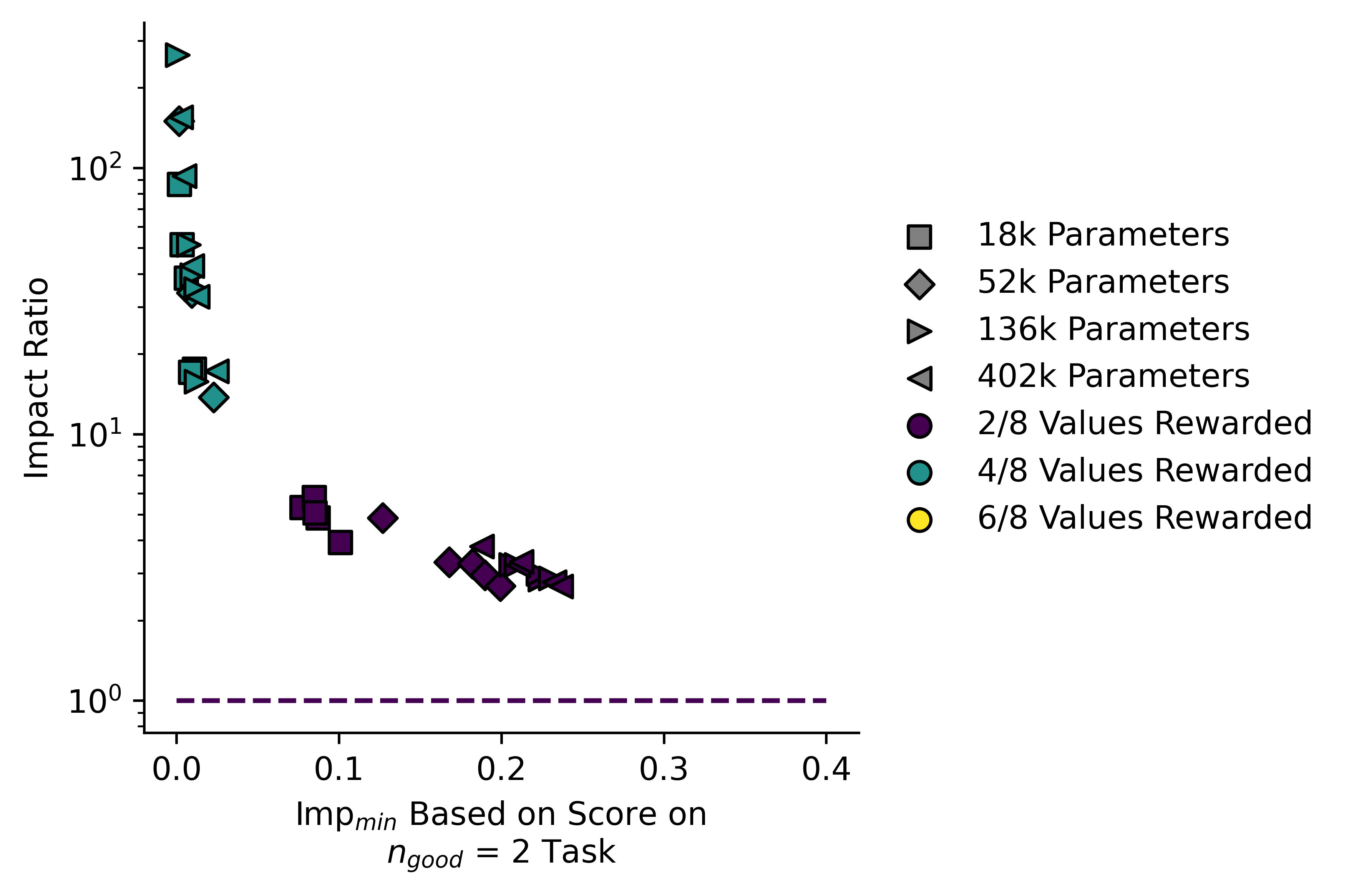
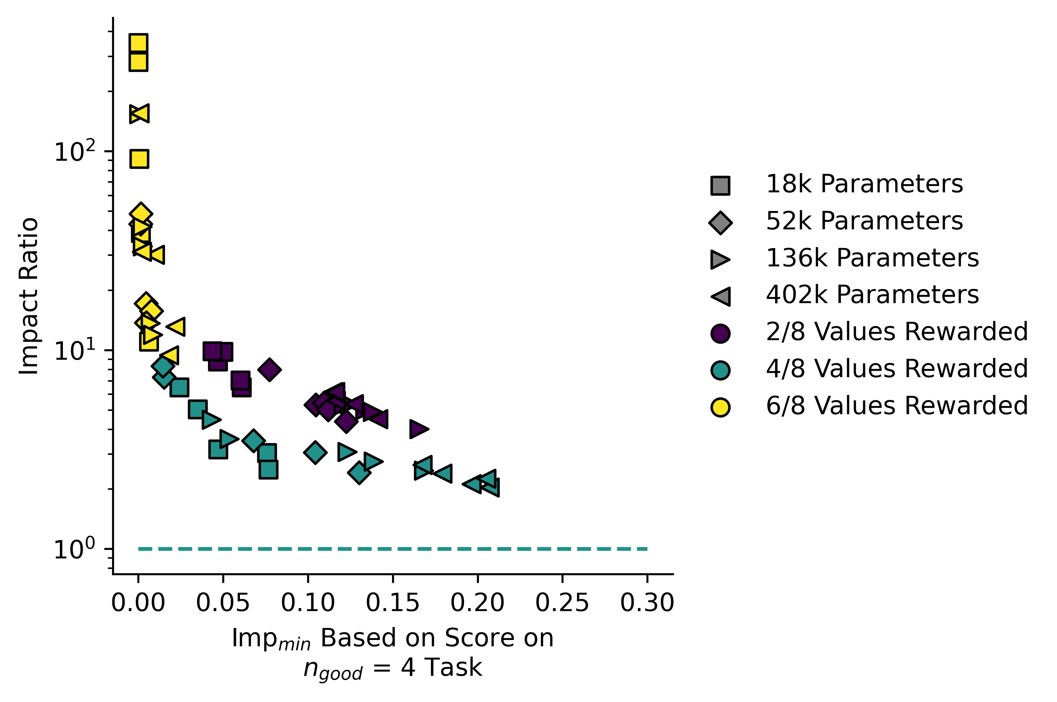
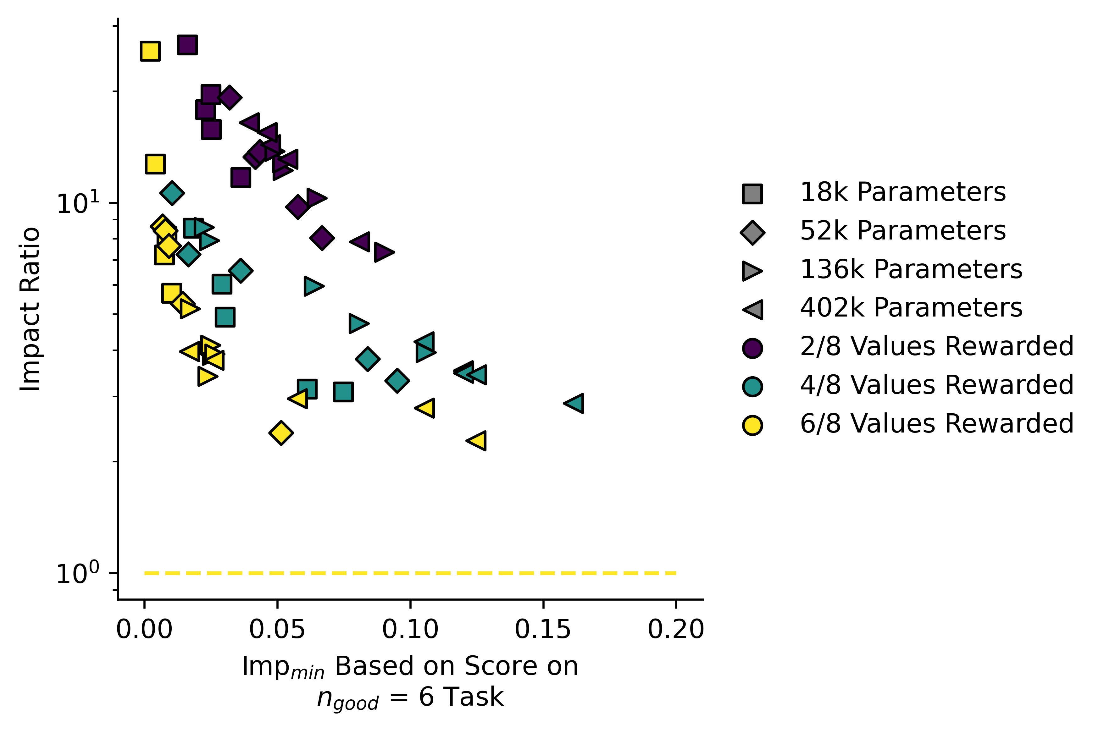
Here I plotted "Excess Impact" $Imp-{Imp}_{min}$ against $Imp$:

 

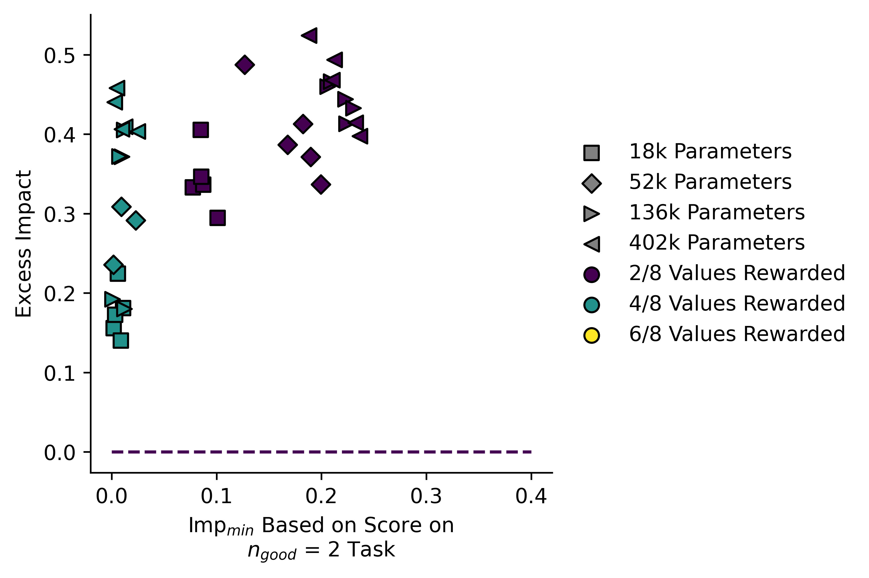
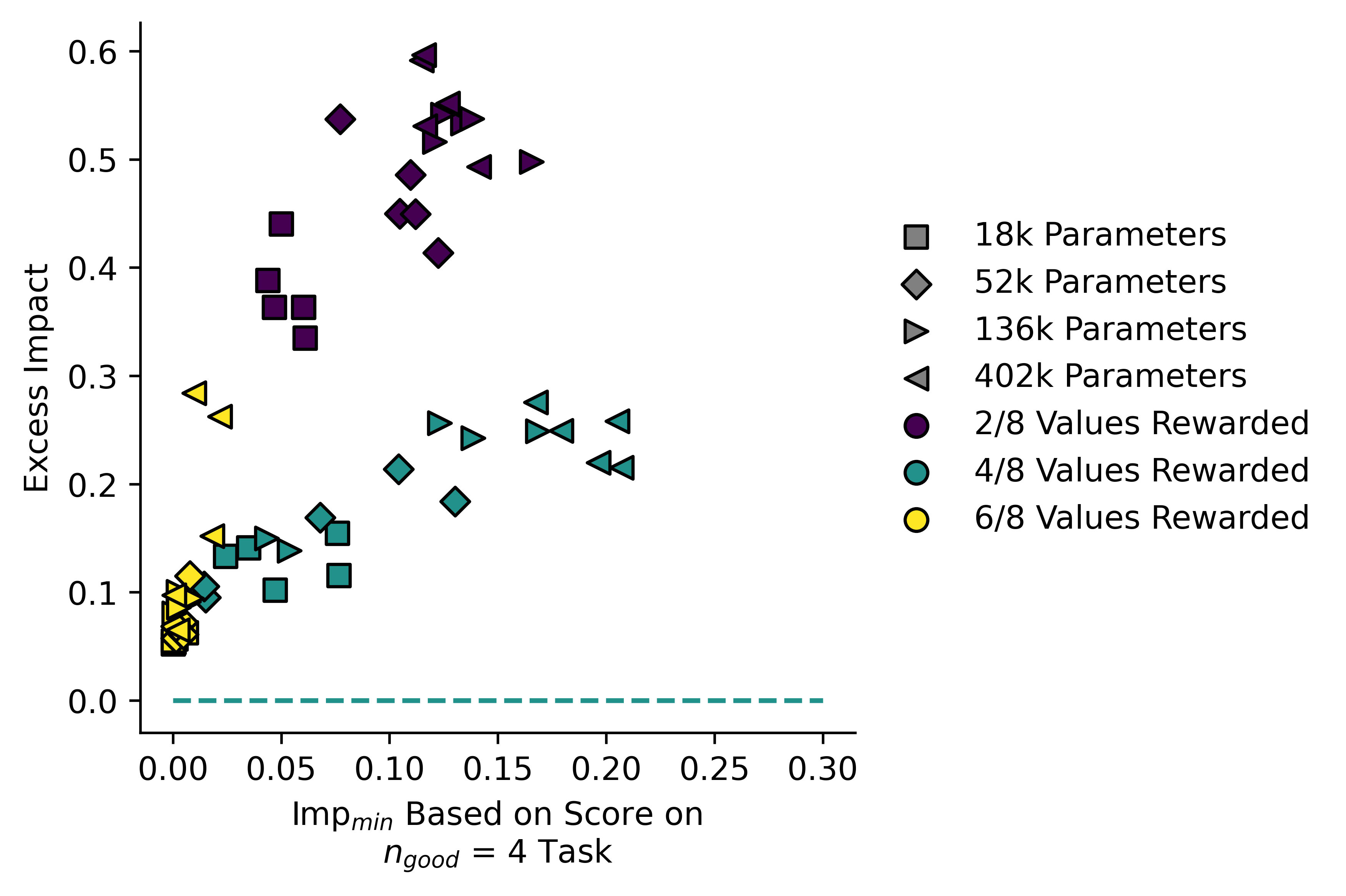
Example training runs from $n_{good}$ = 4

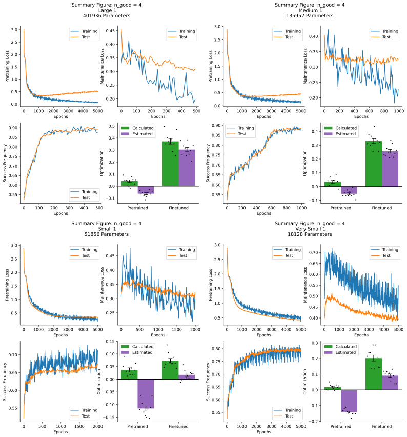
Example figures summarizing training runs:

1. ^{^}

   https://statproofbook.github.io/P/mvn-ltt.html

2. ^{^}

   https://stats.stackexchange.com/questions/60680/kl-divergence-between-two-multivariate-gaussians

3. ^{^}

   https://statproofbook.github.io/P/mean-qf.html

0 comments

Comments sorted by top scores.