Convolution as smoothing

post by Maxwell Peterson (maxwell-peterson) · 2020-11-25T06:00:07.611Z · LW · GW · 5 comments

Contents

  Understanding convolution as smoothing tells us about the central limit theorem
None
5 comments

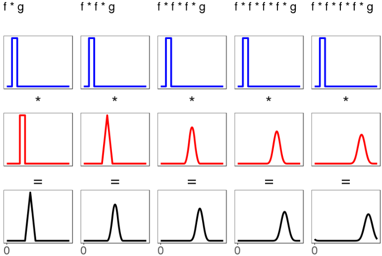
Convolutions smooth out hard sharp things into nice smooth things. (See previous post [LW · GW] for why convolutions are important). Here are some convolutions between various distributions:

(For all five examples, all the action in the functions $f$ and $g$ is in positive regions - i.e. $f\left(x\right)$ > 0 only when x > 0, and $g$ too - though this isn't necessary.) 

Things to notice:

• Everything is getting smoothed out! Even the bimodal case, in the column all the way to the right, has a convolution that looks like it's closer to something smooth than its two underlying distributions are. You might say the spike that uniform $\ast$ uniform gives doesn't seem more smooth, exactly, than the uniform distributions that led to it. But notice the second column, which convolves a third uniform distribution with the result of the convolution from the first column. That second convolution leads to something more intuitively smooth (or if not smooth, at least more hill-shaped). We can repeat this procedure, feeding the output of the first convolution to the next, and each time we get a black result distribution that is a little bit shorter and a little bit wider. Thus we get a smooth thing by repeatedly convolving two input sharp things (f and g):

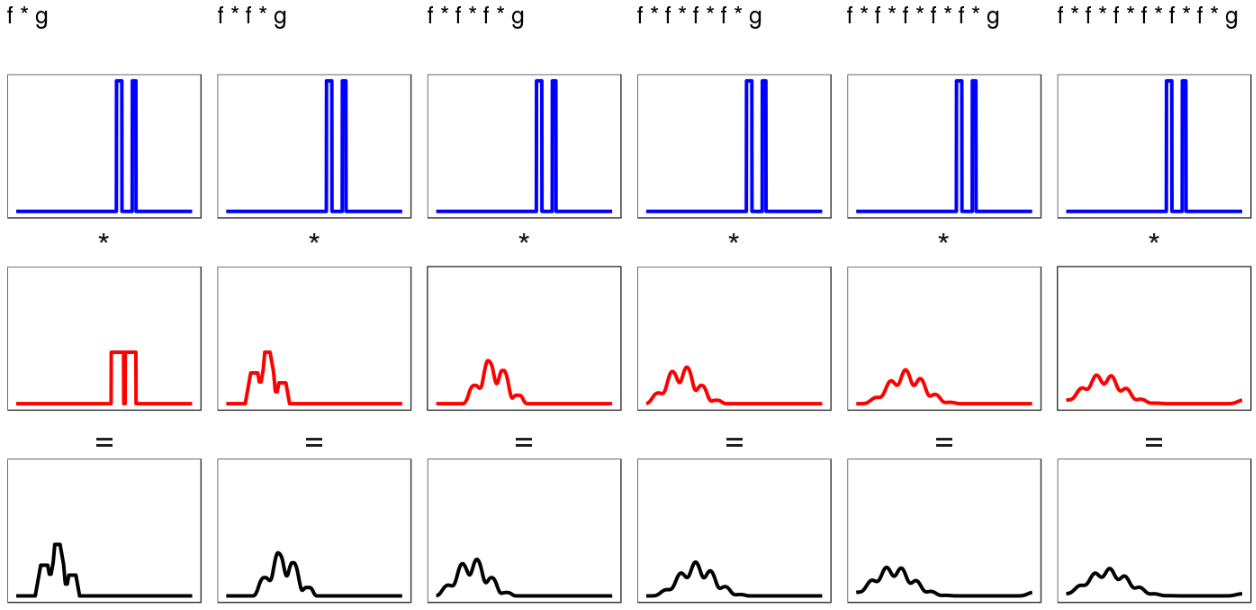
• Even the more difficult bimodal distributions smooth out under repeated convolution, although it takes longer:

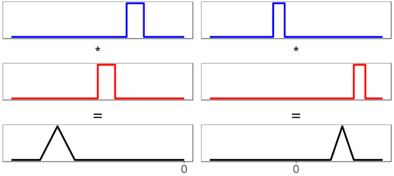
• $f\ast g$ (for positive $f$ and $g$) is always to the right of $f$ and $g$ both. Because all these example $f$ and $g$ are positive, their means are positive. And it's a theorem that the mean $⟨f\ast g⟩$ is always equal to the sum of the underlying means $⟨f⟩+⟨g⟩$. So the location of the distributions is always increasing. Of course, for $f$ and $g$ with negative first moments, the location of $f\ast g$ would go leftward; and if $f$ had negative mean but $g$ had positive mean, the mean of $f\ast g$ could go anywhere. I am actually just describing how addition works, but the idea that you could locate a distribution $f\ast g$ just by summing the locations of $f$ and $g$ was so shocking to me initially that I feel like I should emphasize it.

Understanding convolution as smoothing tells us about the central limit theorem

From Glen_b on stackoverflow:

Convolution acts as a kind of "smearing" operator that people who use kernel density estimation across a variety of kernels will be familiar with; once you standardize the result... there's clear a progression toward increasingly symmetric hill shapes as you repeatedly smooth (and it doesn't much matter* if you change the kernel each time).

(a kernel is like a distribution; italics are mine.)

Up till now I've just called it "smoothing", but convolution on most (all?) probability distributions is better described as a smoothing-symmetricking-hillshaping operation. The graphics above are examples. And remember: The central limit theorem is a statement about convolutions on probability distributions [LW · GW]! So here's a restatement of the basic central limit theorem:

Convolution on probability distributions is a smoothing-symmetricking-hillshaping operation, and under a variety of conditions, applying it repeatedly results in a symmetric hill that looks Gaussian.

Or you could look at it the other way around: The central limit theorem describes what comes out on the other side of repeated convolutions. If someone asked you what the behavior of $D^{\ast }:=d_1\ast d_2\ast d_3\ast \cdots \ast d_n$ was, you could answer with the contents of the central limit theorem. 

Because your answer was the central limit theorem, it would contain information about: how varying the shapes of the component distributions $d_i$ affected the shape of $D^{\ast }$; how many distributions $d_i$ you needed to get close to some target distribution $H$; and what the $d_i$ needed to look like in order for $H$ to look Gaussian. It would also contain the same kind of information for the moments of $H$, like the mean. And the variance. It would describe how to use the skew (which corresponds to the third moment) to evaluate how many distributions $d_i$ you needed for $H$ to look Gaussian (the Berry-Esseen theorem). 

These information, together with various additional conditions and bounds, constitute a network of facts about what kinds of probability distributions $\{d_1,...,d_n\}$ cause $d_1\ast d_2\ast \cdots \ast d_n$ to look Gaussian, and how Gaussian it will look. We call this network of facts "the central limit theorem", or sometimes - to emphasize the different varieties introduced by relaxing or strengthing some of the conditions - the central limit theorems.

---

*: While this kind of thing is true for many distributions, see Gurkenglas in the comments for why we shouldn't take "it doesn't much matter if you change the kernel each time" too literally.

5 comments

Comments sorted by top scores.