Defining Optimization in a Deeper Way Part 4
post by J Bostock (Jemist) · 2022-07-28T17:02:33.411Z · LW · GW · 0 commentsContents
  A Better Thermostat Model
  Point 1: We can Recover an Intuitive Measure of Optimization
  The Lorenz System
  Point 2: Even Around a Stable Equilibrium, Op(A;n,m) an be Negative
  Point 3: Our Measures Throw Up Issues in Some Cases
  Point 4: Our Measures are Very Messy in Chaotic Environments
  Point 5: Op Seems to be Defined Even in Chaotic Systems
  Conclusions and Next Steps
None
No comments
In the last post I introduced a potential measure for optimization, and applied it to a very simple system. In this post I will show how it applies to some more complex systems. My five takeaways so far are:
- We can recover an intuitive measure of optimization
- Even around a stable equilibrium, can be negative
- Our measures throw up issues in some cases
- Our measures are very messy in chaotic environments
- seems to be defined even in chaotic systems
It's good to be precise with our language, so let's be precise. Remember our model system which looks like this:
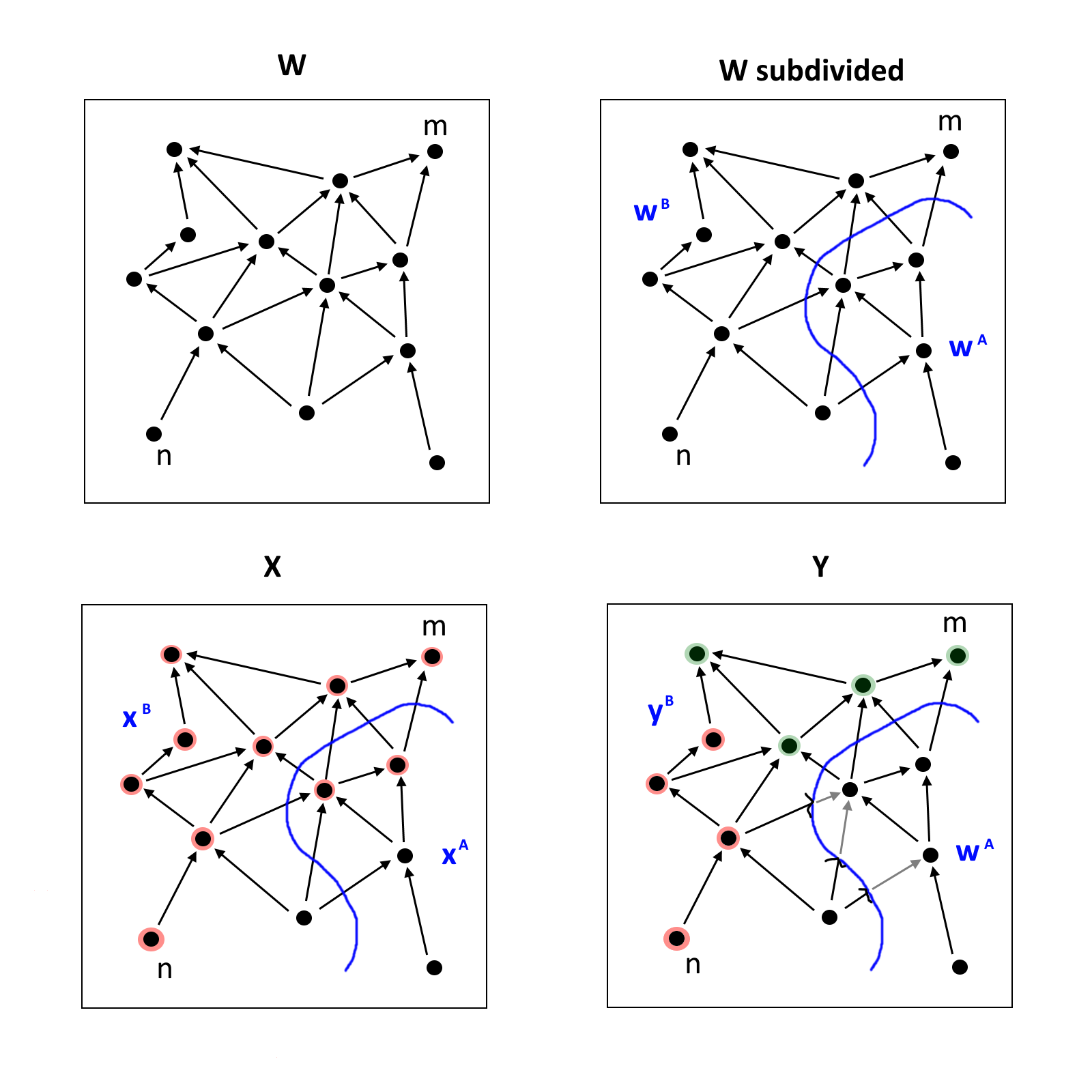
In this network, each node is represented by a real number. We'll use superscript notation to notate the value of a node: is the value of node in the world .
The heart of this is a quantity I'll call , which is:
Which is equivalent to.
( is the generic version of , , )
Our current measure for optimization is the following value:
is positive when the nodes in are doing something optimizer-ish towards the node . This corresponds when is < 1. We can understand this as when is allowed to vary with respect to changes in , the change that propagates forwards to is smaller.
is negative when the nodes in are doing something like "amplification" of the variance in . Specifically, we refer to optimizing with respect to around the specific trajectory , by an amount of nats equal to . We'll investigate this measure in a few different systems.
A Better Thermostat Model
Our old thermostat was not a particularly good model of a thermostat. Realistically a thermostat cannot apply infinite heating or cooling to a system. For a better model let's consider the function
Now imagine we redefine our continuous thermostat like this:
Within the narrow "basin" of , it behaves like before. But outside the change in temperature over time is constant. This looks like the following:
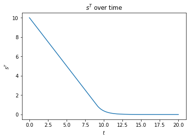
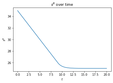
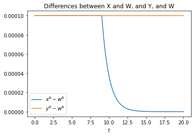
When we look at our optimizing measure, we can see that in while remains in the linear decreasing region, . It only increases when reaches the exponentially decreasing region.
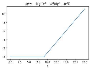
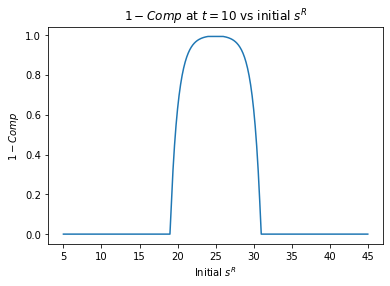
Now we might want to ask ourselves another question, for what values of is positive for a given value of , say ? Let's set , and the initial . The graph of this looks like the following:
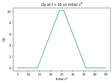
Every initial which has a trajectory which leads into the "optimizing region" between the temperatures of 24 and 26 is optimized a bit. The maximum values are trajectories which start in this region.
Point 1: We can Recover an Intuitive Measure of Optimization
What we might want to do is measure the "amount" of optimization in this region, between the points and , with respect to . If we choose this measure to be the integral of , we get some nice properties.
It (almost) no longer depends on , but depends linearly on .
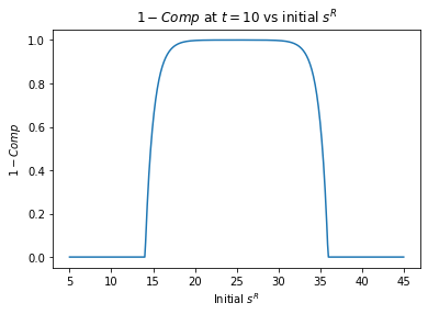
, gives an integral of
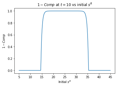
, gives an integral of
, gives an integral of
As , our integral remains (pretty much) the same. This is good because it means we can assign some "opimizing power" to a thermostat which acts in the "standard" way, i.e. applying a change of each time unit to the temperature if it's below the set point, and a change of each time unit if it's above the set point. And it's no coincidence that that power is equal to .
Let's take a step back to consider what we've done here. If we consider the following differential equation:
It certainly looks like values are being compressed about by per time unit, but that requires us to do a somewhat awkward manoeuvre: We have to equivocate our metric of the space of at with our metric of the space of at . For temperatures this can be done in a natural way, but this doesn't necessarily extend to other systems. It also doesn't stack up well with systems which naturally compress themselves along some sort of axis, for example water going into a plughole.
We've managed to recreate this using what I consider to be a much more flexible, well-defined, and natural measure. This is a good sign for our measure.
The Lorenz System
This is a famed system defined by the differential equations:
(I have made the notational change from the "standard" in order to avoid collision with my own notation)
Which can fairly easily and relatively accurately be converted to discreet time. We'll keep as constant values. For values of we have a single stable equilibrium point. For values we get three stable equilibria, and for values we have a chaotic system. We'll investigate the first and third cases.
The most natural choices for are all of any one of the or values. We could also equally validly choose to be a pair of them, although this might cause some issues. A reasonable choice for would be the initial value of either of the two , , or which aren't chosen for .
Point 2: Even Around a Stable Equilibrium, an be Negative
Let's choose , which means we have a single stable point at . Here are plots for the choice of as the set , and as the axis along which to measure optimization. (So we're changing the value of and looking at how future values of and change, depending on whether or not values of are allowed to change)
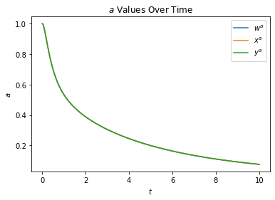
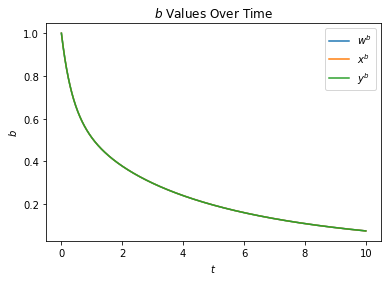
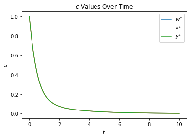
Due to my poor matplotlib abilities, those all look like one graph. This indicates that we are not in the chaotic region of the Lorenz system. The variables , , and approach zero in all cases.
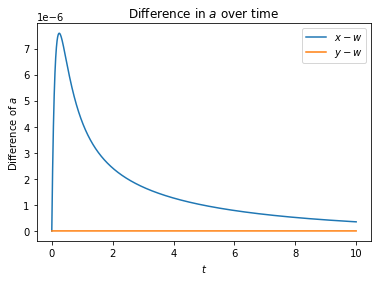
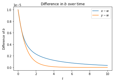
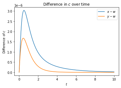
As we can see, difference is greater than the difference . The mathematics of this are difficult to interpret meaningfully, so I'll settle with the idea that changes in , , and in some way compound on one another over time, even as all three approach zero. When we plot values for we get this:
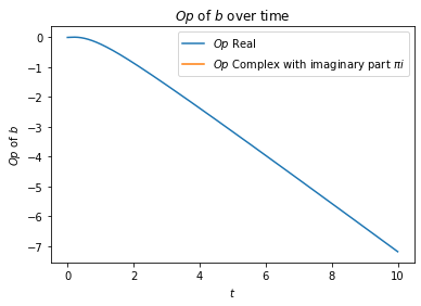
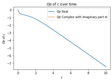
The values for and are negative, as expected. This is actually really important! It's important that our measure captures the fact that even though the future is being "compressed" — in the sense that future values of , , and approach zero as — it's not necessarily the case that these variables (which are the only variables in the system) are optimizing each other.
Point 3: Our Measures Throw Up Issues in Some Cases
Now what about variation along the axis ?
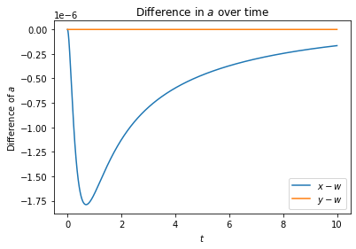
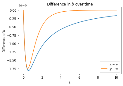
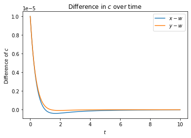

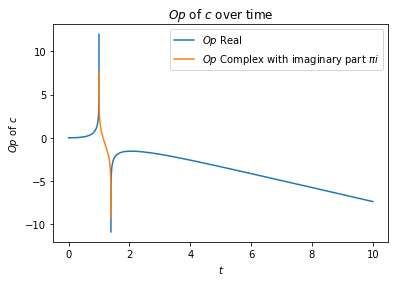
We run into a bit of an issue! For a small chunk of time, the differences and have different signs. This causes to be complex valued, whoops!
Point 4: Our Measures are Very Messy in Chaotic Environments
When when choose , it's a different story. Here we are with as , as the axis of optimization:
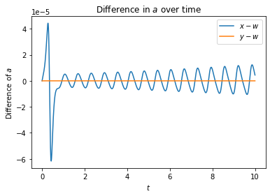
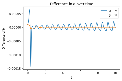
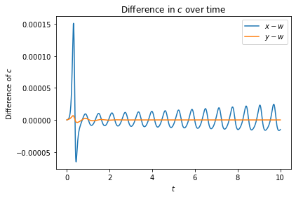
Now the variations are huge! And they're wild and fluctuating.
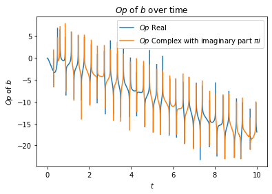
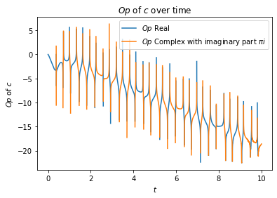
Huge variations across everything. This is basically what it means to have a chaotic system. But interestingly there is a trend towards becoming negative in most cases, which should tell us something, namely that these things are spreading one another out.
What happens if we define as ? This means that for values with we allow a difference between the and values. We get graphs that look like this:
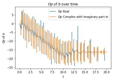
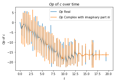
This is actually a good sign. Since only has a finite amount of influence, we'd expect that it can only de-optimize and by a finite degree into the future.
Point 5: Seems to be Defined Even in Chaotic Systems
It's also worth noting that we're only looking at an approximation of here. What happens when we reduce the by some amount? In our other cases we get the same answer. Let's just consider the effect on .
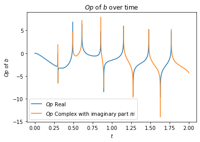
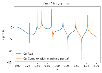
Works for a shorter simulation, what about a longer one?

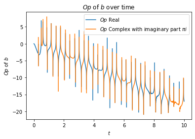
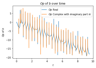
This seems to be working mostly fine.
Conclusions and Next Steps
Looks like our system is working reasonably well. I'd like to apply it to some even more complex models but I don't particularly know which ones to use yet! I'd also like to look at landscapes of and values for the Lorenz system, the same way I looked at landscapes of the thermostat system. The aim is to be able to apply this analysis to a neural network.
0 comments
Comments sorted by top scores.