Polarization is Not (Standard) Bayesian

post by Kevin Dorst · 2023-09-16T16:31:14.227Z · LW · GW · 6 comments

This is a link post for https://kevindorst.substack.com/p/polarization-is-not-standard-bayesian

Contents

  Martingale updating
  What martingale means for polarization
  Why partisans increasingly agree on (some) claims
  Generalizing the argument
  What does this mean?
None
6 comments

TLDR: Standard rational models can explain many aspects of polarization. But not all. Ideological sorting implies that our beliefs often evolve in predictable ways, violating the “martingale property” of Bayesian belief-updating. Rational models need to reckon with this.

---

Polarization is everywhere. Most people seem to think it’s due largely to irrational causes. I think they’re wrong. But today I want to focus on a different disagreement.

Because there’s been a surge of recent papers arguing that polarization may be due to rational causes.^[1]

These papers show that many of the qualitative features of polarization—such as persistent disagreement, divergent updating, etc.—are to be expected from standard Bayesian agents.

There’s a lot I like about these papers. But I think they undersell the hurdles rational theories are facing: real-world polarization is deeply puzzling in a way that (standard) Bayesian models can’t explain.

In particular: what needs to be explained is how polarization could be predictable: because we’ve become ideologically sorted—by geographical, social, and professional networks—we can often predict the way our opinions will develop over time. This violates what’s known as the martingale property (aka the “reflection principle”) of Bayesian updating: your prior beliefs must match your best estimate of your later beliefs.

I’ve given versions of this argument before, but here I’d like to give a (hopefully) better one. The upshot: rational explanations of polarization need to look beyond standard models.

Martingale updating

First: what is the martingale constraint on belief-updating?

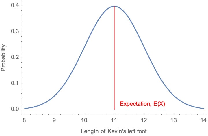
Suppose you’re a Bayesian with a prior distribution P. For any quantity (“random variable”)—say, X = the length of Kevin’s left foot—you can use your priors to form an expectation for the value of X: a probability-weighted average of the possible values of X, with weights determined by how likely you think they are. Perhaps you have a distribution like the following:

 

That’s a pretty boring quantity. But if you’re a Bayesian, your priors encode expectations about any quantity—including the quantity X = what probability you’ll assign to __ in the future.

Suppose I’ve got a coin that’s either (1) Fair or (2) 70%-Biased toward heads; you’re currently 50-50 between these two possibilities: P(Fair) = 0.5 and P(Biased) = 0.5. I’m going to toss the coin once and show you the outcome. Consider the quantity:

P*(Fair) = how likely you’ll think it is the coin is fair, after observing the toss.

You’re currently unsure of the value of this quantity. After all, the coin might land heads, in which case you’ll lower your probability of Fair (heads is more likely if it’s biased toward heads). Or the coin might land tails, in which case you’ll raise your probability of Fair (tails is more to be expected if Fair than if Biased). Since you have opinions about how likely it is you’ll see a heads (tails), you can use these to form an expectation for your future opinion about whether the coin is fair, i.e. P*(Fair).

Martingale updating is the constraint that your current probability of Fair must equal your current expectation for your future probability [LW · GW] of Fair: P(Fair) = E[P*(Fair)].^[2]

Since we know you’re currently 50%-confident the coin is fair, we can infer from this that your current expectation of your future probability in Fair must also equal 50%. Let’s check. (If you trust me, skip the math.)

How likely do you think it is the coin will land heads? Since you’re 50-50 between the chances being 50% (if Fair) and 70% (if Biased), your current probability in Heads a straight average of these: 60%.^[3]

Given this, we can use Bayes theorem to figure out how much your probability in Fair will shift if you see a heads (or a tails), and then use that to calculate the expectation.

If you see the coin land heads, then you’ll shift to 5/12 ≈ 41.7%-confident that it’s fair.^[4]

And if you see the coin land tails, you’ll shift to 5/8 = 62.5%-confident that it’s fair.^[5]

Since you’re 60% (=3/5) confident in Heads, that means your current expectation for your future probability in Biased is:

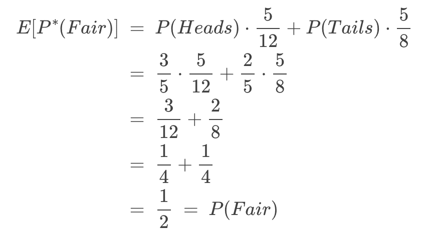
That worked.

Here’s a mathematical rule of thumb: if you plug in random-looking numbers and you get an equality coming out, there’s a good chance that equality holds generally.

It does. This is due to the fact that Bayesians defer to their future opinions: conditional on their better-informed future-self having a given opinion they adopt that opinion.

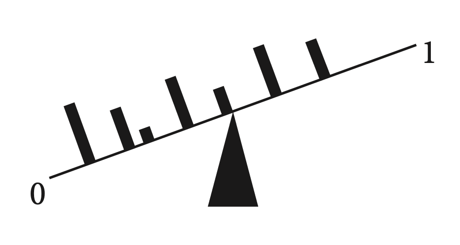
You can think of it as if they are pulled toward those possible future opinions. Imagine we have a bar labeled ‘0’ on one end and ‘1’ on the other, with a fulcrum representing your current probability:

Now we add weights corresponding to your possible future opinions. If your future-self might adopt probability ½ for the proposition, we put a weight halfway along the bar (and so on). The heaviness of the weights correspond to how likely you currently think it is that your future-self will adopt that probability. This will tip the scale:

To balance it, we need to move your current probability (the fulcrum) to the center of mass (equivalently: the expectation) of the weights:

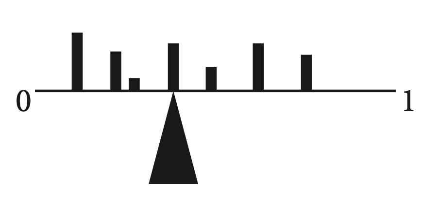
Thus, if you’re a (standard) Bayesian, your current probability always matches your best estimate of your future probability.

What martingale means for polarization

Martingale forbids a Bayesian’s beliefs from moving in a predictable direction. But polarization makes it so that our beliefs often move in predictable directions. Standard Bayesianism can’t explain this.

To get an intuition, suppose Nathan starts out politically unopinionated, but is about to move to a liberal university in a liberal city. If he knows anything about politics, he should know there’s a good chance this will make him more liberal—after all, college does that to a lot of people, especially moderates:

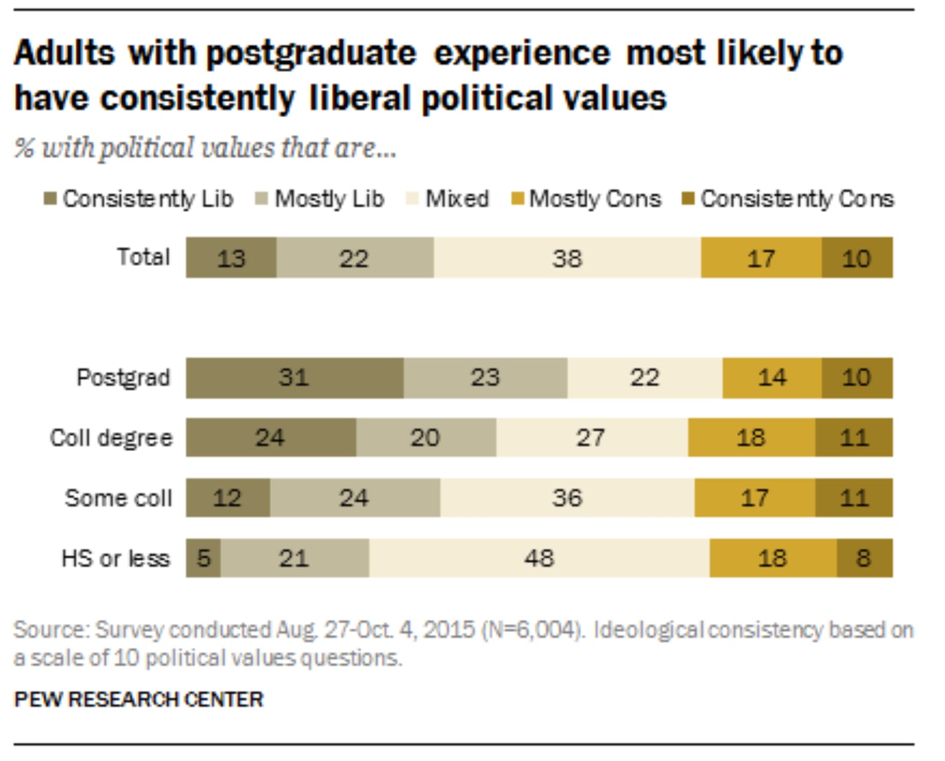
So it looks like he should “expect”, if anything, to become more liberal.

But you might think this is too quick. After all, a decent proportion of people who go to college become more conservative—16.8% according to one study (vs. 30.3% becoming more liberal). So Nathan definitely shouldn’t be sure he’ll become more liberal.

That’s consistent with a martingale failure—all we need is that on average, across possibilities he leaves open, he’ll become more liberal. But it does make it much harder to prove that people violate martingale in forming their political opinions.

I think we can prove it using ideological sorting.

Why partisans increasingly agree on (some) claims

It’s common to say that polarization has led us to disagree more and more. And obviously there’s a sense in which that’s true—the US has become increasingly ideologically sorted over the past few decades. For example, the proportion of people who adopt across-the-board liberal (or conservative) positions grew dramatically between 1994 and 2014:

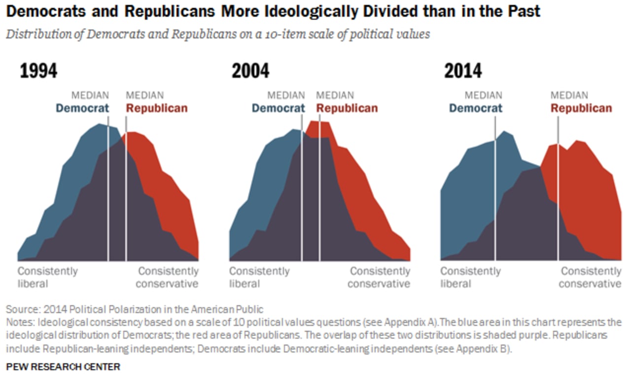
What does this mean? In 1970, you couldn’t predict someone’s opinions about gun rights from their opinions on abortion rights; now you can. So Republicans and Democrats disagree more consistently than ever before, right?

Sort of. But what’s often overlooked is that this implies that there are also claims that partisans increasingly agree about.

In particular, if we line up a string of partisan-coded claims (Abortion is wrong; Guns increase safety;…) then since most people either accept or reject all of these claims together, that means that most people will agree that these claims stand or fall together: they are either all true, or all false.

Precisely: Republicans believe both A (Abortion is wrong) and G (Guns increase safety), Democrats disbelieve both A and G. It follows that they both believe the (material) biconditional: “Either abortion is wrong and guns increase safety, OR abortion is not wrong and guns don’t increase safety”. (That is: “(A&G) or (¬A&¬G)”; equivalently, A<–>G.)

We don’t need any empirical studies to establish this; it’s a logical consequence of being confident (or doubtful) of both A and G that you’re confident of the biconditional.^[6]

We can turn this into an argument against Standard-Bayesian theories of polarization.

First, an intuitive case. Suppose Nathan is about to immerse himself in political discourse and form some opinions. Currently he’s 50-50 on whether Abortion is wrong (A) and on whether Guns increase safety (G). Naturally, he treats the two independently: becoming convinced that abortion is wrong wouldn’t shift his opinions about guns. As a consequence, if he’s a Bayesian then he’s also 50-50 on the biconditional A<–>G.^[7]

He knows he’s about to become opinionated. And he knows that almost everyone either becomes a Republican (so they believe both A and G) or a Democrat (so they disbelieve both A and G). Either way, they’re more confident in the biconditional than he is. He has no reason to think he’s special in this regard, so he can expect that he’ll become more confident of it too—violating martingale.

For example, suppose:

• He’s at least 40%-confident that he’ll become a Republican, and so become 70%-confident that both A and G are true: P(P*(A&G) ≥0.7) ≥ 0.4.
• He’s at least 40%-confident that he’ll become a Democrat, and so become at least 70%-confident that both A and G are false: P(P*(¬A&¬G)≥0.7) ≥ 0.4.

It follows that he violates martingale: his expectation for his future probability of the biconditional is 56%, while his current probability is only 50%.^[8]

Generalizing the argument

The natural objection to this argument is that maybe Nathan shouldn’t treat A and G independently. Even though he sees no direct connection between the two, perhaps his knowledge of political demographics should make him suspect an indirect one: He thinks, “If Abortion is wrong, that means Republicans are more likely to be right about things—so it’s more likely they’re right about other things, like guns.” Etc.

If he thinks this way, it’ll raise his initial probability for the biconditional above 50%—potentially recovering the martingale property.

But we can give a much more general argument that pretty much anyone whose politically unopinionated will violate martingale.

Suppose now that Nathan begins with some—any—degrees of confidence in each of A and G: P(A) and P(G). He also has some—any—opinion about how (non)independent they are; this is their covariance relative to his priors:

(If c = 0, he treats A and G independently.)

The argument has two premises. The first:

P1 (No Expected Conspiracy): Nathan doesn’t expect to later come to think that A and G are more anti-correlated than he currently does.

(Formally: his current expectation for his future covariance for A and G is as high as his current covariance: E[Cov_P*(A,G)] ≥ Cov_P(A,G) = c.^[9])

This seems obviously correct. If anything, Nathan expects to come to think that A and G are more positively correlated than he does now, as he comes to understand the subtle interrelations between political issues more deeply.

For P1 to be violated, he’d have to know that even though people’s beliefs about abortion and guns tend to pattern together, he is likely to become increasingly confident that if abortion is wrong, then guns don’t increase safety. That’s bizarre. (The most natural possibility is for him to lack any directional expectation about the shifts in his opinions about A and G’s relevance: E[Cov_P*(A,G)] = Cov_P(A,G).)

Second premise:

P2 (Correlated Posteriors): Nathan currently expects his future opinions about A and G to be positively correlated.

(Formally: his covariance for his future opinions is positive: Cov_P(P*(A),P*(G))>0.^[10])

This seems obviously correct too: after all, he knows that most people’s opinions about A and G pattern together. Even though he can’t be sure how his opinions will shift, he currently thinks that if he become more confident that abortion is wrong, he’s probably drifting in a Republican direction, so it’s more likely that he’ll become confident that guns increase safety.

I think most people who are about to become politically opinionated in our current culture will satisfy these two premises. They are enough to prove a martingale failure.

We do this by “reductio”: supposing martingale were satisfied, we prove a contradiction—so martingale can’t be satisfied. In particular, even if Nathan doesn’t violate martingale for A or for G, he’s still guaranteed to violate it for the biconditional A<–>G. (The proof is in a footnote.^[11])

What does this mean?

One of the core features of real-world polarization is that people’s opinions are predictably correlated. This makes premises like P1 and P2 applicable, meaning that they violate martingale. And that, in turn, implies that their updating process can’t be a Standard-Bayesian one.

What to make of this?

First, explanations of polarization must be able to account for martingale failures. This is a serious limitation of many theories.

Second, martingale is often thought to be the central rationality-constraint of Bayesianism—thus there’s a case to be made that insofar as martingale violations drive polarization, it must be due to irrationality.

But third: there’s another way. Provably, Bayesians who satisfy standard rationality constraints (the “value of information”) will violate martingale if and only if they have higher-order uncertainty: if and only if they’re rational to be unsure what the rational opinions are.

This, I think, is the key to understanding polarization. But that’s an argument for another time.

---

If you liked this post, subscribe to my Substack to get future ones.

1. ^{^}

   A non-exhaustive sampling: Jern et al. 2014, Cook and Lewandowsky 2016, O’Connor and Weatherall 2018, Benoît and Dubra 2019, Henderson and Gebharter 2021, Nielsen and Stewart 2021, Pallavicini et al. 2021, Melnikoff and Strohminger 2023.

2. ^{^}

   E[X] is your probability-weighted average for the values of X:

3. ^{^}

   By total probability:

4. ^{^}

   By Bayes Rule:

   

5. ^{^}

   By Bayes Rule:

   

6. ^{^}

   In fact, empirical studies on this would likely be confounded by conversational and signaling effects of agreeing to odd statements of the form “Abortion is wrong if and only if guns are dangerous”.  That English sentence conveys a connection between the two, whereas the material biconditional which we’re trying to assess does not.

7. ^{^}

   P(A<–>G) = P((A&G) or (¬A&¬G)) = P(A&G) + P(¬A&¬G) = 0.25 + 0.25 = 0.5.

8. ^{^}

   Note that P*(A&G)≥0.7 and P*(¬A&¬G)≥0.7 each imply that P*(A<->G) ≥ 0.7.  Since they are disjoint possibilities and his probability in each is at least 40%, it follows that his probability in their disjunction is at least 80%, so P(P*(A<–>G)≥0.7) ≥ 0.8. By the Markov inequality, E[P*(A<–>G)] ≥ P(P*(A<–>G)≥0.7)* 0.7 ≥ 0.8*0.7 = 0.56 > 0.5 = P(A<–>G).

9. ^{^}

   Unpacking definitions, this says:

   

10. ^{^}

    Equivalently: E[P*(A)P*(G)] > E[P*(A)]•E[P*(G)].

11. ^{^}

    For reductio, suppose martingale holds: for all propositions X, E[P*(X)] = P(X). Then:

    

6 comments

Comments sorted by top scores.