A primer on machine learning in cryo-electron microscopy (cryo-EM)
post by Abhishaike Mahajan (abhishaike-mahajan) · 2024-12-22T15:11:58.860Z · LW · GW · 0 commentsThis is a link post for https://www.owlposting.com/p/a-primer-on-ml-in-cryo-electron-microscopy
Contents
  Introduction
  Why do cryo-EM?
    The alternatives
      X-ray crystallography
      Nuclear Magnetic Resonance (NMR)
  Why cryo-EM is better
  The cryo-EM workflow
    Sample preparation
    Imaging
  Reconstruction
  Some machine learning problems in the area
    Conformational heterogeneity
    Ab initio reconstruction
    Compositional heterogeneity
  What’s left?
None
No comments
(7.9k words, 36 minutes reading time)
Note: thank you to Jason Kaelber, a professor at Rutgers University and director of their cryo-EM facility, for commenting on drafts of this essay! Also thank you to Surge Biswas, the founder of Nabla Bio, for answering questions I had over cryo-EM.
Introduction
Cryo-electron microscopy (cryo-EM) has been gaining increasing popularity over the past few years. Used as a way to perform macromolecular structure determination for decades, cryo-EM really hit its stride around 2010, when it crossed the resolution thresholds needed to determine protein structures. The technique was so deeply powerful, so able to answer biological questions for which no alternative tool existed, that its creators were awarded the 2017 Nobel Prize in chemistry.
But I wasn’t really aware of that when I first stumbled across cryo-EM.
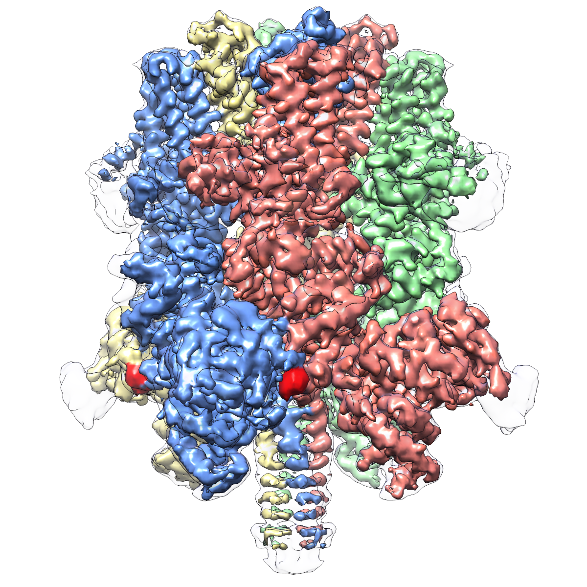
My initial thought was that it was a cool-sounding name, and the output of the process made for similarly cool images.
Weird looking, isn’t it?
I first came across cryo-EM as a concept via Ellen Zhong (a machine learning professor at Princeton) in 2022. Because she co-wrote what has become one of my favorite papers of all time, I was also interested in what else she had worked on. But very much unlike my favorite paper, which had to do with viral language models, almost all of her work had to do with applying ML to cryo-EM.
This was weird! Cryo-EM wasn’t something I ever saw much. While, admittedly, I was entirely ignorant of the field until 2022, it still felt like it wasn’t a very popular topic. Most people seem to work in small molecule behavior prediction or antibody modeling or something you’d see dozens of papers about at a NeurIPS workshop.
Cryo-EM feels almost like…pure physics or chemistry, something that distinctly wasn’t an ML problem. As such, I mentally tossed it away as something beyond my mental paygrade. But I kept seeing more and more cryo-EM news.
More cryo-EM papers from Zhong’s lab.
Gandeeva Therapeutics raising $40M in 2022 to do drug discovery work using ML-assisted cryo-EM.
There was something going on here, something important.
Yet, there are shockingly few resources on how to learn about this field, starting from the ground up. I’ve written technical introduction for molecular dynamics, toxicology, and antibody engineering before. All of those felt like I was rehashing a collection of a dozen-or-so review papers, just phrased in a way I found more appealing.
But here…there’s almost nothing, outside of maybe Zhong’s PhD thesis. I hope to add to that body of work.
This essay will first explain the alternatives to cryo-EM, why cryo-EM exists at all, and why so many people seem to be interested in it. Then we’ll move into how cryo-EM works, including sample prep, imaging, and reconstruction. Then we’ll finally be ready to approach how people are throwing ML at the problem to both solve fundamental issues with cryo-EM and, most interestingly, extend it beyond what people originally thought it was capable of.
Lots to go through. Let’s start!
Why do cryo-EM?
Cryo-EM is a method to understand the three-dimensional structure of extremely small structures: proteins, small molecules, and so on. It shares this categorization with (primarily) two others of note: X-ray crystallography and nuclear magnetic resonance (NMR) imaging. It’s worth going over them first before we discuss the advantages of cryo-EM.
But this post is only meant to deeply discuss cryo-EM and I’d like to avoid turning this essay into a textbook, I won’t deeply cover the other two, only a very quick overview of how it works, their advantages, and disadvantages.
The alternatives
X-ray crystallography
X-ray crystallography is one of the most established methods of protein characterization, having existed in prototype forms since the early 1900’s. The technique involves purifying and crystallizing the target molecule, arranging it into a highly ordered, repeating lattice structure. When X-rays are directed at the crystal, they are scattered by the electrons in the atoms, producing a diffraction pattern. This pattern is then mathematically transformed into an electron density map, from which the atomic model of the molecule can be built.
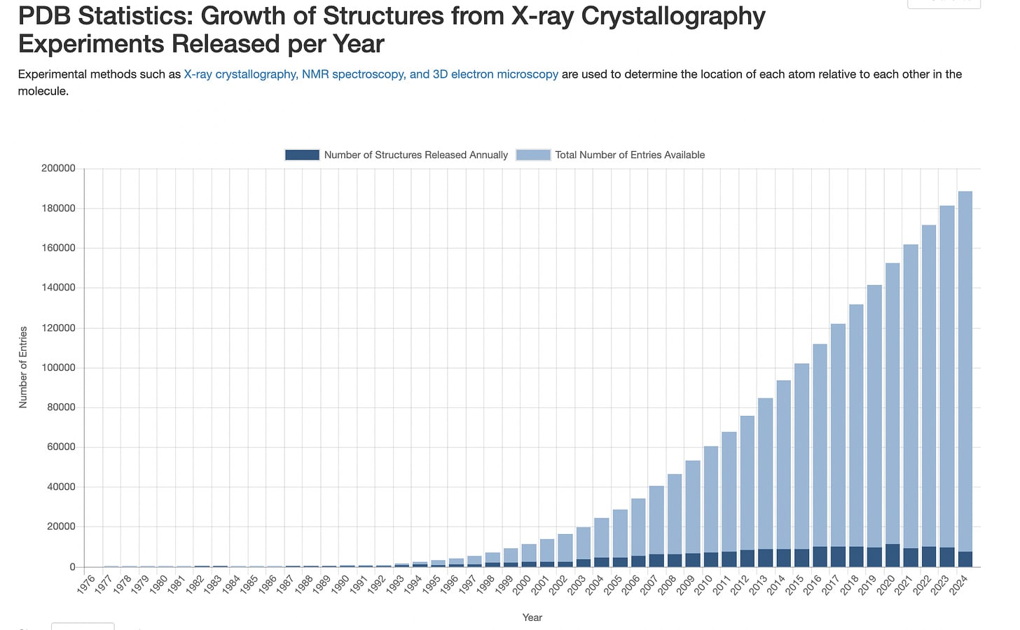
There are lots of benefits to the method. It can achieve extremely high resolution (often below 1 Å) and has well-established protocols and analysis methods backed by decades of research. As such, this method has been responsible for solving the vast majority of protein structures in the Protein Data Bank.
Unfortunately, the need for crystallization is a huge problem. For one, large protein complexes are nearly impossible to crystallize at all, and large complexes are one of the most understudied parts of our biology. Two, crystalizing a protein implies you’ll be fixing it in place. In turn, this means that any measurement of the resulting structure will captures a single, static image of the crystallized molecule, missing out on any alternative conformations.
Nuclear Magnetic Resonance (NMR)
NMR spectroscopy is a departure from crystallization, instead relying on purified molecules placed in a solution, typically water. The technique exploits the fact that certain atomic nuclei behave like tiny magnets. When these atoms are placed in a powerful magnetic field, they can absorb and release specific frequencies of radio waves. By precisely controlling the magnetic field and sending carefully timed pulses of radio waves, researchers can measure how atoms within a molecule interact with each other. From this, researchers can gather information about the distances and angles between atoms, allowing them to calculate a set of possible structures consistent with the observed interactions.
Because you're eschewing crystallization, NMR allows one to study protein motion. As in, you can observe dynamic changes in protein structure, protein-protein interactions, and even study partially unfolded states. NMR can also provide information about protein dynamics on various timescales, from microseconds to seconds. Of course though, the utility of these coarser timescales is suspect.
NMR has one particularly strong limitation. The technique is generally limited to relatively small proteins (typically under 50 kDa), as larger proteins produce increasingly complex spectra that become difficult to interpret. This turns out to be a major enough problem that NMR is the least used structure characterization method in the PDB.
Why cryo-EM is better
First and most importantly, cryo-EM doesn't require crystallization of studied-protein structures. Instead of forcing proteins into a crystal lattice, researchers instead flash-freeze them in a thin layer of vitreous ice (something we’ll discuss more later). The benefit of this is that we can study massive protein complexes, membrane proteins, and other structures that have historically been nearly impossible to crystallize. The size advantage of cryo-EM works in the opposite direction of NMR — larger structures are often easier to work with in cryo-EM than smaller ones. While NMR struggles with anything over 50 kDa, cryo-EM excels at massive molecular machines like ribosomes (~2,500 kDa) or virus particles (often >1,000 kDa). At those sizes, even X-ray crystallography struggles. Again though, cryo-EM has a problem with smaller structures, which we’ll expand on more later.
Another major advantage is that cryo-EM can capture proteins in multiple conformational states simultaneously. You may intuitively guess that flash-freezing proteins would present the same ‘static-only-structures’ problem as crystallization, but this actually turns out to not be true in practice. Why exactly this is the case requires some more explanation, so we’ll get to that later.
Finally, resolution was historically cryo-EM's weak point — for many years, it couldn't match the atomic detail provided by X-ray crystallography. The primary bottleneck was that detecting electrons passed through flash-frozen protein was difficult, but better detection setups — circa 2020 — changed that. Nowadays. modern cryo-EM can regularly achieve resolutions better than 3 Å, and in some cases even approach 1 Å resolution. Close to X-ray crystallography levels!
Of course, there isn’t a free lunch here. Cryo-EM struggles in one particular area: ease of performing it.
For one, electron microscopes themselves can run in the seven figures to acquire, and that’s before considering the specialized equipment (liquid nitrogen or liquid helium) needed to run it. Secondly, dealing with cryo-EM data is monstrously challenging. Data artifacts will naturally arise from the inevitably noisy freezing process, extracting conformations from electron diffractions is difficult at best, and atomic resolution can be inconsistent across a structure.
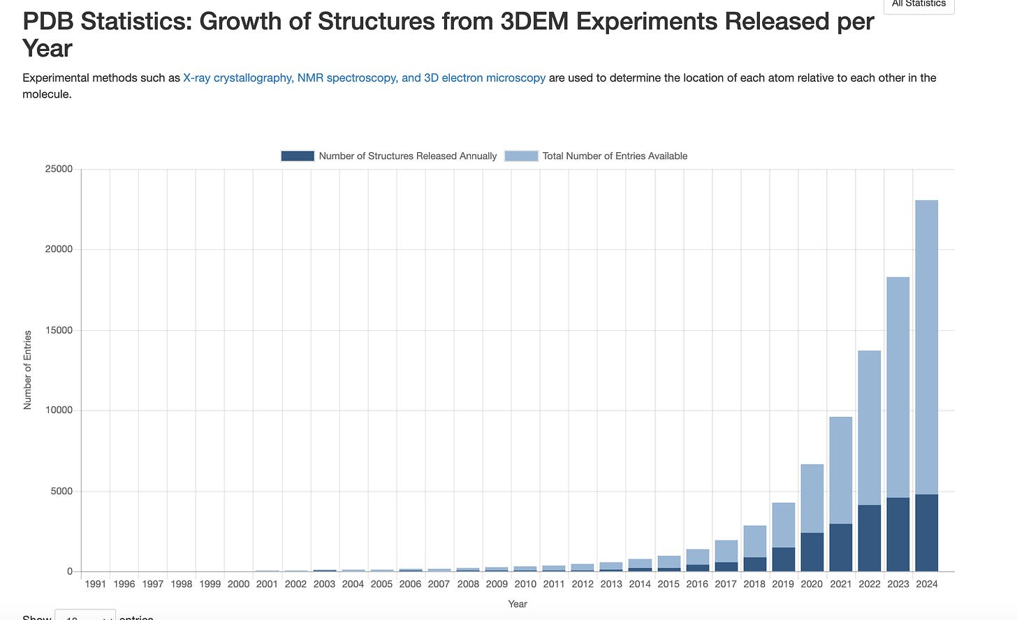
Likely amplifying the prior issues, the final problem here is that cryo-EM is a reasonably new characterization method. Of course, ‘new’ is relative. Cryo-EM had its first characterized structure in 1991, whereas X-ray crystallography had it in 1958. Though one would expect this 33 year lead time to have been washed out in the 30~ years since, it is likely that the relative inaccessibility of cryo-EM has made research on it difficult.
This all said though, as the chart below shows, cryo-EM is picking up speed with each passing year!
Of course, there’s still aways to go, comparing it to X-ray crystallography structures:
With this surface-level overview, we should be ready to start poking at how cryo-EM works at all. We’ll first explore sample preparation (preparing our protein for input to the cryo-EM grid), then how the imaging process works (via the electron microscope), and then discuss how typical protein structure reconstruction works.
The cryo-EM workflow
Sample preparation
Let’s assume you have a purified solution of proteins, suspended in some aqueous solution. This is nontrivial to do, especially with large protein complexes that cryo-EM is known to excel at, but it’s a complexity we’ll ignore for now.
What’s next?
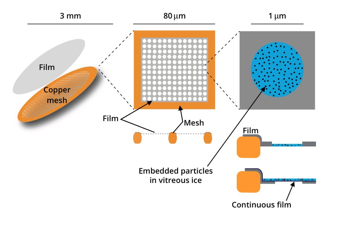
First, we squeeze out the protein solution onto a grid. What does the grid look like? Here’s a picture:
From here. Focus on the first two images, ignore the left-most one for now.
Basically, it’s a small metal mesh (usually copper) that's been covered with a thin film of carbon. The carbon film — similar to the copper mesh it’s on top of — isn't a solid sheet, it's full of holes, typically arranged in a regular pattern. The whole copper grid is only about 3mm in diameter, and each hole in the carbon film is just a few hundred nanometers across. So you end up with each hole of the copper grid itself containing many grids of the carbon film.
There’s lots of commercial variety here; everything from the hole sizes to the thickness of the carbon sheets can be altered. There’s a great deal of nuance here w.r.t why you’d prefer some parameters over others, but we’ll ignore it for now. If you’re interested, this topic is a whole field in of itself called ‘grid optimization’.
One more question: why a grid…of grids? It’s hard to answer right now, we’ll come back to that later, let’s move on.
When we apply our protein solution to this grid, it creates thin films across these holes, like a soap bubble spanning a bubble wand. So, can we start imaging right away? Not yet, there’s one problem: biological molecules like proteins are mostly made of light elements — carbon, nitrogen, oxygen, hydrogen. These elements don't interact very strongly with electrons. When you shoot an electron beam through a ‘naked’ protein, almost all the electrons go straight through without being deflected. In other words, proteins are nearly invisible to electron beams.
One curious side note before we move on: the electron argument makes sense for why ‘naked’ proteins won’t work, but I assumed there was another reason too for why naked proteins won’t work. The electron microscope we'll eventually use operates in a near-vacuum — it has to, or the electrons would just bounce off air molecules instead of hitting our sample. And I assumed vacuums are extraordinarily unfriendly to biological samples, so they must be…protected in some way. But I stumbled across a paper with an insane title (The fate of proteins in outer space) that disproved this:
Many proteins, and many protein-protein complexes, retain their structural integrity in vacuo, at least for a sufficiently long time, for many of their essential structural features to be retained and be capable of study in intimate detail.
Either way, imaging naked proteins is infeasible. What can we do?
One way could be to cover the proteins with heavy elements and image that! This is what used to be done with via chemical staining of the protein film. Here, you first deposit a fine layer of heavy metal salts on the surface of your grid to allow electron interaction and then throw electrons at that. And, practically speaking, so-called negative-staining is still often done in the earliest stages of a cryo-EM project to assess feasibility. Unfortunately, the application of the aforementioned salts can both limit resolution (as the deposition of the salts prevents fine-grained imaging) and can cause artifacts in the final structure.
Is there any other way we can we make the protein visible?
As the name ‘cryo-EM’ may suggest, the answer is to freeze the proteins. You’d be forgiven for thinking that this is deeply unintuitive. If our whole problem with imaging naked proteins is that they don’t interact with electrons well, what do we gain from surrounding the protein in a frozen matrix of water, which is made of even lighter elements than proteins, and then shooting electrons at them?
The answer is a bit of a bait-and-switch; while proteins are indeed nearly invisible to electrons, ice is even more invisible to electrons. You can think of ice here as offering a way to create a nice ‘background’ state from which we can more clearly make out the protein structure. A more scientific way to put this wouldn’t be ‘invisible’ or ‘not invisible’, but rather that the electron is phase shifted by its passage through the object — one consistent level of shift when passing through ice, and another varied set of shifts as it passes through the protein. And we obviously can’t use the liquid water, since, again, our electron microscope needs a vacuum to work, so liquids would instantly boil. As such, ice.
This might seem like a small distinction— using ice as a background rather than using heavy metals as a foreground — but it turns out to be really important. When we use heavy metals in negative staining, we're really creating a mold around the protein, like pressing a coin into clay. While this gives us good contrast, it also means we're not really seeing the protein itself, just its outline. With ice, we're actually seeing the protein itself suspended in mid-air, the fuzziness of its view being brought into more clarity via a consistent background (the ice).
To note though, normal ice here won’t work. When you turn water into ice, it naturally wants to form crystals. This process, called nucleation, starts when a few water molecules happen to arrange themselves in an ice-like pattern. Once that happens, other water molecules are recruited to join into the pattern.
This crystallization is a problem for two reasons.
First, when water molecules arrange themselves into ice crystals, they literally take up more space than they did as liquid water. This expansion can tear proteins apart or change their conformation (notably, this particular effect of ice nucleation is why stuff like human cryonics is really hard; shoutout to Cradle, a startup that is trying to solve this problem!). This is obviously antithetical to our lofty imaging goals.
Second, while ice itself doesn’t scatter electrons, ice crystals do, which will ruin the otherwise nice contrast we had with our protein.
Is it possible to have ice without the ice crystals?
Yup! It turns out that ice crystals will not form if water is frozen to −135 °C at a rate of around 100,000 degrees Celsius per second. If water is frozen that fast, ice nucleation crystals will literally not have time to form. To achieve this rate of freezing, people typically dunk the copper grid into liquid ethane. I’ve attached some interesting notes about this in the footnotes, but we’ll move on.[1]
How is this all done? There’s a dedicated machine for it, called the Vitrobot! There’s a video on the process here.
Finally, with all that, let’s assume we’ve gotten our copper grid frozen, our proteins now stuck in a layer of vitreous ice across our copper grid. We’ve succeeded! Keep in mind though that we’ve blown past a lot of complexity here. Sample preparation in cryo-EM is a huge field, and what I’ve written here doesn’t do it justice at all. But hopefully it gives you a good mental model.
Same picture as before, now just look at the right-most image.
Now, we just remove the grid from our vat of liquid ethane/nitrogen, store it in a bucket of liquid nitrogen (to keep it cool), and move it on over to the electron microscopy. It’s time to start imaging!
Imaging
The workhorse here will be a transmission electron microscopy, or TEM. It may be helpful to have the whole process plainly explained at the start, and we’ll walk through the steps.
- Load up the sample into the TEM.
- The TEM will shoot a beam of electrons at our sample.
- These electrons travel through our frozen protein sample.
- Most electrons pass straight through the ice.
- Some get deflected by the protein.
- An electron detector at the bottom records where all the electrons ended up.
This is actually pretty simple. It’s not too dissimilar to brightfield micrography, where visible light is shown beneath a sample, and we look from above to see what structures show up. In this case, the deflector is the ‘eye’.
First up, imaging, which will occur on a grid-by-grid level. Before we start explaining imaging, it may be good to note that how imaging is done is the answer to the previous question of why have grids at all: each grid is a ‘shot’ at having a potentially good image. If some holes have ice that's too thick or thin, or if the protein distribution or orientation isn't ideal in some areas, we can simply move on to other holes. This grid pattern essentially gives us thousands of independent attempts at getting good images from a single sample preparation.
Now that we know the purpose of the grid, we can ask an even more fundamental question: why is there a carbon grid on top of the carbon grid? Let’s leave that one to the footnotes.[2]
Moving on, taking advantage of this grid setup, cryo-EM imaging typically occurs in three steps: grid-view, square-view, and hole-view. The hope of this is to quickly discard unpromising sections of the grid and focus in on the higher-quality sections. In order:
- In grid view, we take a low magnification "atlas" of the entire grid. This will immediately show us if we've got usable ice. If the ice is too thick, we'll barely be able to see through the grid squares at all. Usually, we’ll see a gradient of ice thickness across the grid, so we’ll have options for finding the perfect thickness for imaging.
- In square-view, we examine individual copper grid squares at medium magnification. This is where we can spot all sorts of potential problems — crystalline ice (bad!), contamination, or even more subtle variations in ice thickness.
- Finally, hole-view, where we zoom in to actually look at individual holes in the carbon film. These are also often referred to as micrographs. This is where we're hoping to see a nice, even distribution of our proteins — not too crowded, not too sparse. If we're not seeing what we want at this level, we go back to sample prep.
From here. This shows grid, square, and hole views, in order.
Notably, the electron energy stays roughly constant at 300 keV throughout this whole process, only the magnification changes. One thing to ponder is this 300 keV number; how safe is that for imaging? Are we expecting it to damage our protein? Generally, yes, to the point where it can dramatically alter the structure of our proteins. There’s a broader collection of work here in tuning the electron energy, but we’ll ignore that.
This whole process is automated in modern microscopes, which can systematically work through these levels, collecting thousands of images over days of operation.
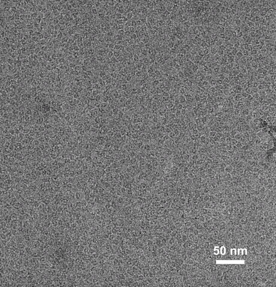
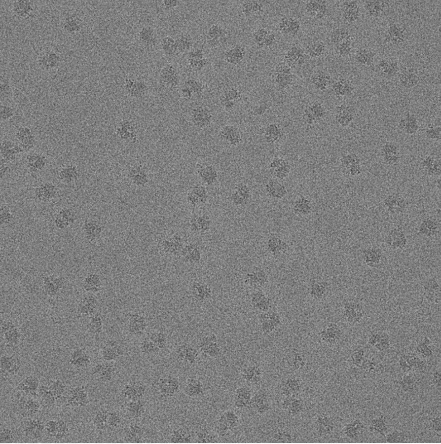
What does an ideal hole-view look like? Like this:
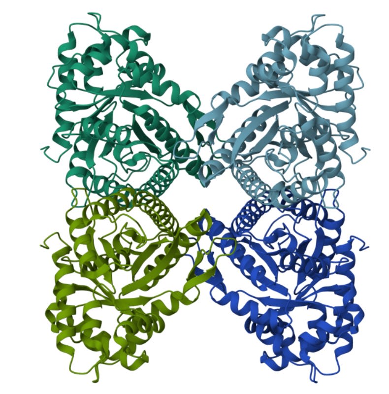
Each of the little dark-ish blobs is an aldolase particle, an enzyme involved in energy production. What does that look like in ribbon-form? Here’s the derived ribbon structure from that blob:
Hmm. There’s a bit of a difference.
So we've got our blobs. Thousands of them, each a 2D snapshot of our protein frozen in ice. And somehow, we need to turn this into those into a 3D dimensional structure. How?
Reconstruction
Consider this:
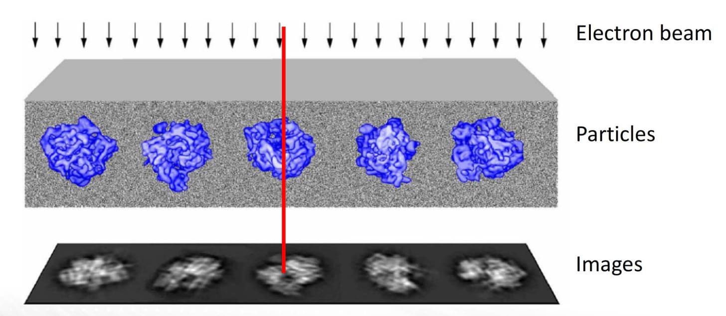
When we covered our grid with a purified solution of proteins, we don't naively expect them to order themselves in any particular direction. Their orientation will, usually, be random! And it turns out that this randomness is actually a feature, not a bug. Why? Because if every protein landed in exactly the same orientation, we'd only ever see it from one angle. Instead, we get thousands of different views of the same structure. Like so:
Now, you may say, ‘while the particles may not be perfectly ordered, it isn’t at all obvious that the orientations will be uniformly random.’. This is correct! The tendency for particles to arrange themselves in a specific pattern is referred to as ‘orientation bias’, or ‘preferred orientation’, and is actually one of the biggest problems involved in actually running cryo-EM. For the purposes of this essay, we’ll pretend that this isn’t an issue, since most of the fixes have to do with either the sample prep or imaging process, such as this, and I am even less equipped to comment on that than the current topic of this essay.
Thus, our job can be phrased as the following: given thousands of these (assumed random) 2D views, each one capturing a different angle of a 3D structure, reconstruct the 3D dimensional structure.
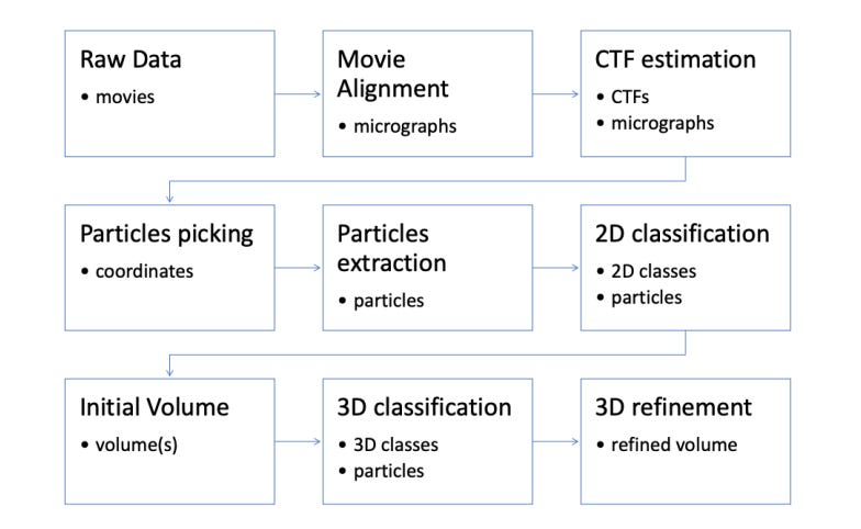
How do you do this? Like this:
Let’s ignore the top column. CTF estimation is an interesting subject that I’d recommend reading up on, but its…a bit disconnected from everything else we’ve been discussing and requires more background information.
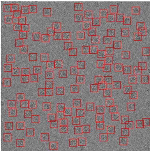
The second step is something called particle picking (which basically also encapsulates particle extraction). Before we get to actual 3D reconstruction, we need to visually isolate the good proteins. Remember, the noise-signal ratio in these micrographics is absolutely awful; many of the proteins here will be degraded, ice thickness will vary, the micrographics may have contaminates, and so on. We need to pluck out the segments of every micrograph that are promising and focus in on those.
In practice, particle picking relies on either template matching (user-predefined particles as templates for identifying particles in micrographs through image matching), or just training an image bounding-box model for identification of good particles via manual curation of a training set. Either way, it seems like it’s a deeply annoying process to do. It seems like the process is close to being fully automated, but, circa 2024, there are still papers being published on New and Improved methods for doing it, so I imagine there’s still ways to go.
Anyway, here’s what a final set of particles may look like, highlighted in a red box.
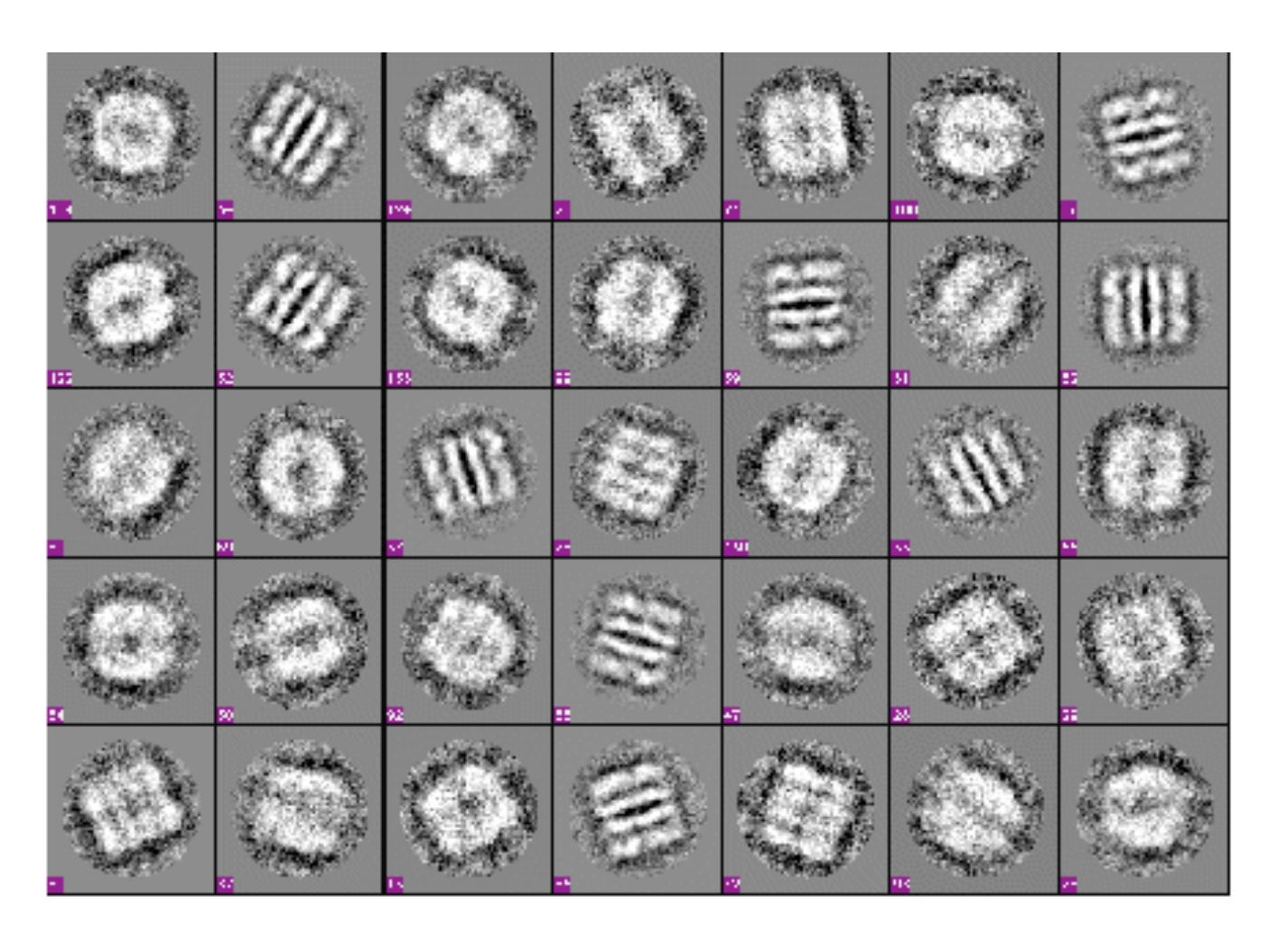
From here, we can move onto 2D classification. We’d ideally like to cluster our particles such that we have, e.g, 20 particles that are taken from the same view, another 20 that are taken from another view, and so on. The hope is that each of these groups are maximally different from one another on a pixel-by-pixel level, such that each group, if merged, can offer a ‘class average’. For example, in the image below, each row-column image shows one class average.
Why do this classification step at all? For the same reason we did atlas imaging and particle picking; we want to bump up the signal-to-noise ratio as much as possible. After this, we’ll end up with a set of class average images, a limited set of 2D views into what our 3D protein actually looks like.
Now what? We have three things left: defining the initial volume, 3D classification, and 3D refinement. The following paragraphs will be concerned with all these three topics at once, so I’ll stop calling out individual items.
Also, it’s at this point in a lot of cryo-EM lectures that you’ll need to start applying Fourier transforms to your class average to fumble your way towards reconstruction of the 3D shape. Truthfully, relatively little of that makes immediate sense to me, so let’s start off with staying in the pure image world, and then slowly motivate why turning to the frequency space makes sense. If you’d like to learn this specific area more deeply, you should check out Dr. Grant Jensen’s videos.
The first challenge is that we need some starting point — some initial guess at what our 3D structure might look like. This is the "initial volume" problem. There are a few ways to approach this, but, in the most ideal case, we have a 3D structure that already roughly looks like our protein. Obviously, this leads to a kind of chicken-and-egg problem. In practice, you can also rely on something less well structured: partial structures, low-resolution structures, and so on. But a pretty good structural prior is, unfortunately, necessary to do cryo-EM. In the machine learning section of the essay, we’ll discuss ways you can get around this requirement.
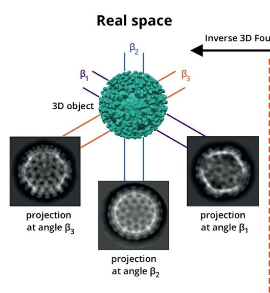
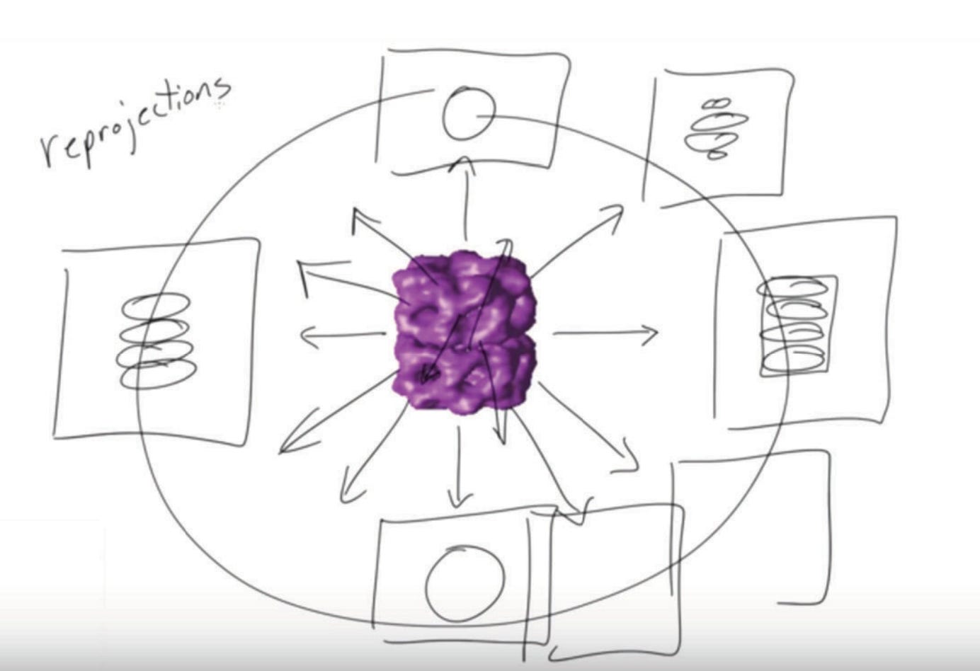
Once we define this initial volume, we’ll perform what are called ‘reprojections’ of this volume. Across every angle of the initial volume, shown in purple, we’ll simulate the 2D projection of that initial volume.
Now what? This:
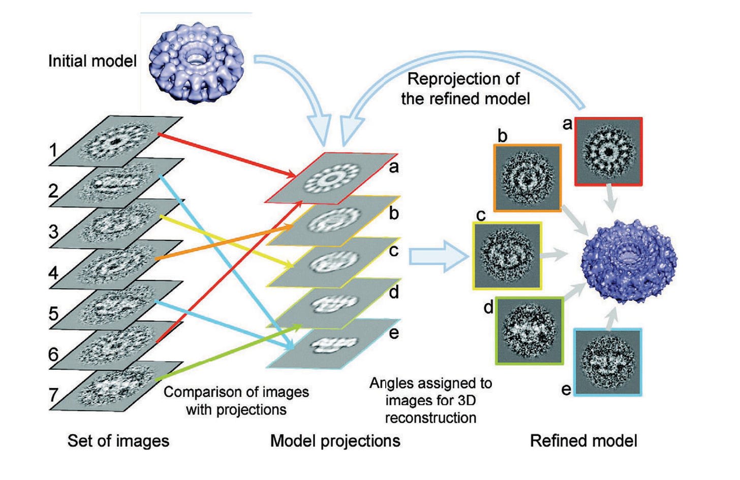
On the left, we've got our "Set of images" (labeled 1-7) — these are our class average 2D images in our sample. They're noisy and blurry, but you can see they're all showing the same structure from different angles.
In the middle, we have "Model projections" (labeled a-e). These are simulated 2D views generated from our initial 3D model (that blue donut-shaped thing at the top). Obviously, these are artificially clean but serve as good ‘ground truths’ for what a 2D image from a given angle should look like.
From here, we simply take every class average particle and compare them to every one of the model reprojections. For the closest matching reprojection, we average the reprojection with the class average! And if multiple class averages are close to the same reprojection, we simply take the average of those class averages alongside the reprojection! Slowly, we replace each reprojection via this averaging process.
Then, because we know our initial model that created the reprojections, it is mathematically simply to alter the 3D initial model to reflect the modifications of the reprojections. After the first round, we expect a slightly better 3D structure. And then you simply repeat!
Each round gets us closer to the true structure, and you simply continue until you’re satisfied with the final structure! There’s also a version of this that uses expectation maximization, which is what is used in practice, but we’ll ignore that for now.
Notably, this is why cryo-EM structures look blobby and semi-artifactual. We’re basically stretching and shrinking a pre-existing blob! Reusing the same picture from the start:
Now, importantly, we’ve thus far been operating only in the 2D image domain. But in practice, cryo-EM 3D refinement occurs in the frequency domain via the Fourier transformation. Why is that?
In real space, if we wanted to figure out how similar two protein images are, we'd need to try aligning them in various ways — shifting them around, rotating them, and comparing pixel by pixel. This is computationally expensive and can be sensitive to noise. When we transform our noisy images into frequency space, we're essentially decomposing each image into a sum of simple wave patterns. Rotations of the protein in real space become simple shifts in frequency space. This means that instead of trying every possible rotation angle to align two images, we can directly compare their frequency patterns. Moreover, the Fourier transform naturally separates different scales of information – low frequencies capture the overall shape of the protein, while high frequencies represent fine details. This separation allows us to work hierarchically, first aligning the basic shapes before trying to match the detailed features.
TLDR: it’s faster and simpler. No reason you couldn’t operate in real space alone though, other than slower to compute!
And that’s about the entire cryo-EM process! Again, obviously I’m skipping a ton of nuance and details here, but this should all give you a decent mental model for how the whole system works. Time to move onto what machine learning problems exist here.
Some machine learning problems in the area
Each of these will be focused on a piece of Ellen Zhong’s work, primarily in the realm of image reconstruction. While there are many researchers in this space, relatively few have touched as many aspects of the ML problems here as her, so we rely on her work alone for convenience.
As is usually the case in my articles, I cannot do justice to every research problem in this area. The focus on reconstruction is partially because that’s the whole point of cryo-EM, so any work there in improving it is pretty high impact. But it’s also because reconstruction is a pretty intuitively understandable topic.
Conformational heterogeneity
The traditional reconstruction methods we discussed earlier assume all these configurations can be averaged into a single meaningful structure. This assumption fails when proteins exhibit significant conformational heterogeneity. And, unfortunately for us, many interesting proteins do indeed demonstrate conformational heterogeneity.
In this case, our 2D projections aren't just different views of the same 3D object — they're different views of slightly different 3D objects. Each image potentially represents a unique conformational state (albeit likely not massively structurally different). The dimensionality of this problem becomes far more immense; naive reconstruction like we were previously doing would simply capture the most common conformation but ignore all the others.
One of Zhong’s most famous papers (and what became her thesis) published in 2020, titled CryoDRGN: reconstruction of heterogeneous cryo-EM structures using neural networks, pokes at this problem.
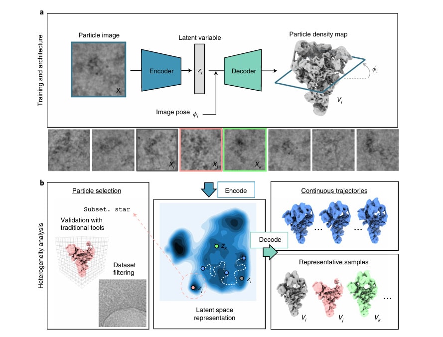
CryoDRGN is a variational autoencoder that, rather than trying to sort particles into discrete classes or approximate them as linear combinations of base structures, will instead learn a continuous generative model of 3D structure via the 2D particles. The model consists of two main components that work together: an encoder network that maps 2D particle images into this latent space, and a decoder network that generates 3D density maps given the latent space.
Training begins with a dataset of particle images and their estimated viewing angles from consensus reconstruction. The core insight here is that we can learn both the conformational states and 3D structures simultaneously by asking: "What distribution of 3D structures could have produced these 2D images?".
During each training iteration:
- The encoder network examines a particle image and predicts where in conformational space (latent space) that particle likely exists
- The decoder network takes that latent space point, alongside its viewing angle, and generates a corresponding 3D structure.
- Wait…how do we get the viewing angle of a particle? Isn’t that unknown? In practice, what the authors do is go through the usual reconstruction process we discussed above and capture an averaged structure that ignores conformational heterogeneity. From there, they use this averaged structure to grab the likely viewing angles of any given particle. This is actually one of CryoDRGN's main limitations (and one they point out in the paper) — it can only work if the conformational heterogeneity isn't so severe that it prevents getting decent angle estimates from homogenous reconstruction.
- This predicted 3D structure is projected to 2D (used a non-machine learned equation) given the pose information.
- The difference between this projection and the actual particle image drives the loss function.
For inference on the training dataset, the encoder network can map all particle image into the latent space, which gives us a distribution showing what conformational states were present in our sample. From there, we can simply use dimensional reduction techniques to learn at all possible conformations that exist in our dataset. There will likely be blobs of major conformations, smaller blobs of rarer conformations, and still yet intermediate state between all of them.
Reconstruction with no assumptions on the level of structural heterogeneity! Well…at least if the heterogeneity isn’t too strong, per my comment on the viewing angles.
One important note that may already be obvious to you (but wasn’t to me upon first reading): CryoDRGN isn’t really a model with weights you can re-use. It has to be retrained again for each new protein! The model hasn’t learnt some generalizable understanding of 2D particles → 3D maps.
Ab initio reconstruction
Because of this demand for the angle of every particle, cryoDRGN still has to deal with the pesky initial volume problem. What if we dropped that requirement entirely? This is often referred to as ‘ab inito reconstruction’; ab initio meaning ‘from first principles’. This would be quite nice; it’d mean that basically no prior information about a set of particles would be necessary to reconstruct it.
Unfortunately, cryoDRGN can’t do that.
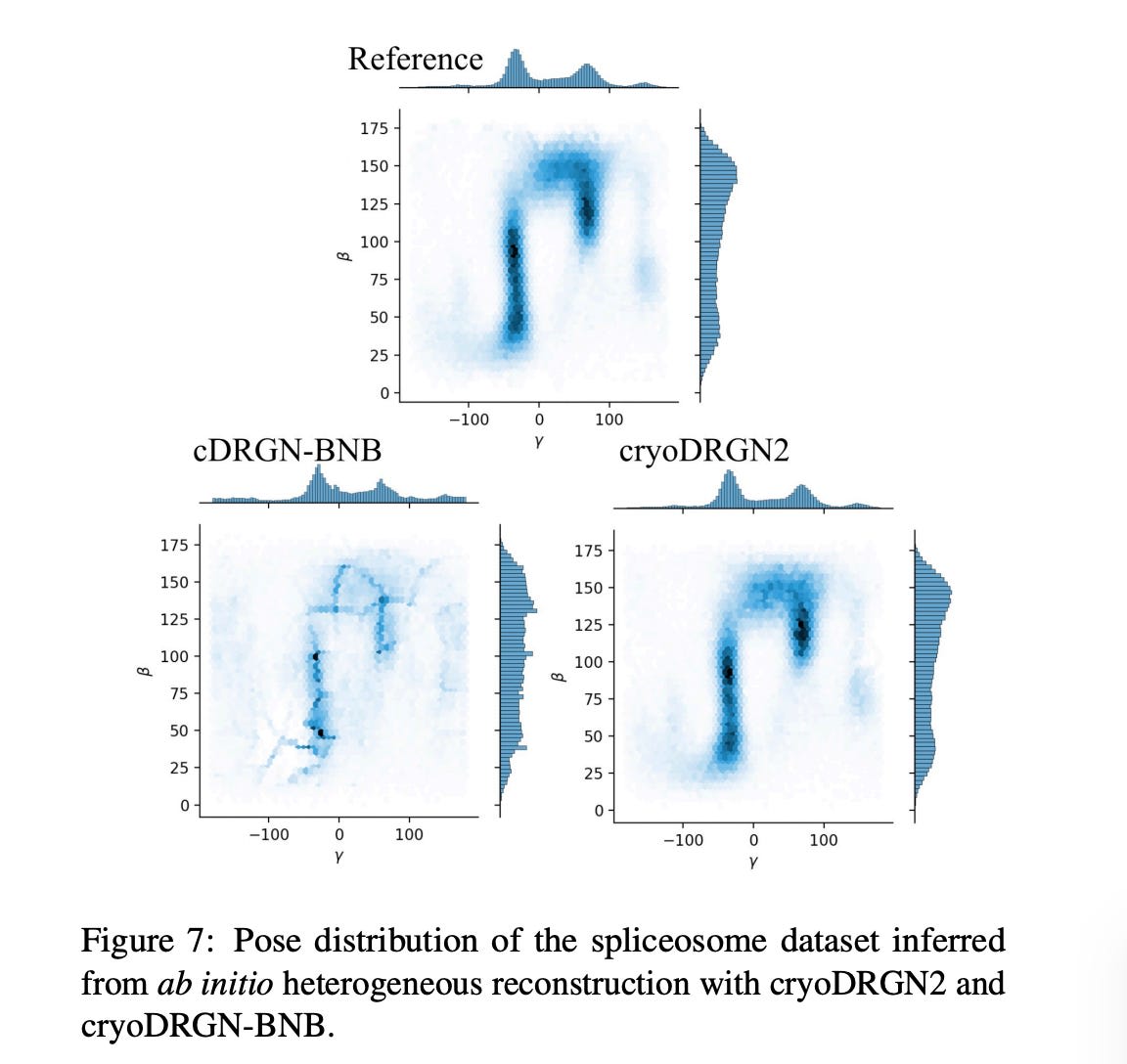
But cryoDRGN2 can! Enter another one of Zhong’s papers, published in 2021: CryoDRGN2: Ab initio neural reconstruction of 3D protein structures from real cryo-EM images.
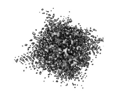
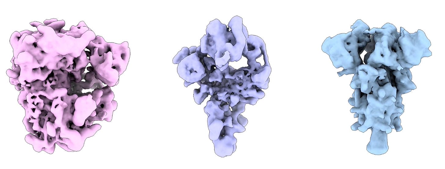
With cryoDRGN, we approximate the result of this search space via the averaged single-conformation structure, and use that to generate an angle pose to feed into the model. With cryoDRGN2, we purposefully eschew this pre-made structure. But…we do need to start somewhere. And that somewhere is in whatever random 3D structure is produced by our untrained neural network with randomly initialized. Perhaps something that looks like this:
Garbage! But we’ll refine it over time.
From here on out, we go through each of our 2D protein particles and try to answer the following question: how does this this particle align with our (terrible) initial model?
How do we do this? First, some context: as you’ll recall, each 2D protein particle could have been taken from any 3D orientation (rotation) and any 2D translation. That's a 5-dimensional search space: 3 dimensions for rotation (SO(3) group) and 2 dimensions for translation (x,y shifts). SO(3) seems obvious, but why (x,y)? Because protein particles aren’t perfectly centered in our bounding boxes; they could be slightly off center.
So, in the brute force case, we’ll simply need to check every single possible re-projection of this initial model across every angle (SO(3)) and every translation (x,y). If we’re splitting up 15° rotation in 3D space, that gives you 4,608 possible rotations, and if you're using a 14x14 translation grid, that's another 196 positions.
That means for each of out thousands particle image, you need to check 4,608 × 196 = 903,168 different possible 2D projections! Bit intractable. They do some tricks to help reduce the computational load of this (though the process is still expensive). Specifically, relying on Fourier spaces and doing ‘frequency marching’, which is where they start by matching low-frequency features and gradually incorporate higher-frequency details. Understanding these optimizations isn’t super useful in my opinion, but worth checking out section 3.2 of the paper if you’d like to know more.
Once we have poses (rotations + translations) for each particle image, we can update our neural network model (which is a simple MLP). This model is in charge of generating 3D structure. We push 2D particles + pose angles through the network and the network outputs a 3D structure, which hopefully should become more and more refined over time. At a certain point, we may say ‘hey, our predicted 3D model is (probably) a fair bit better than this random noise we started off, we should update the poses’, which kicks again kicks off the pose search process from before, updating all of the poses to hopefully be more accurate. Again, this search process is expensive, so we only run it intermittently.
There’s also a ‘model reset’ bit. What’s that? There’s an interesting pathology in cryoDRGN2 where the earliest pose information are useful for very coarse information, but practically useless for finer grained information. But, by the time the 3D structure improves, and the poses get better, such that we should be able to learn higher resolution information, the model has essentially learned to entirely ignore the fine-grained information theoretically contained within our particle image. To fix this, the authors simply reset the model weights and start training from scratch, while still relying on the improved 3D model.
Finally, what do we do during inference? At the end of the training pipeline, we have two things: a refined global structure used to get pose info, and a model capable of generating a possible 3D structure given a new particle. We could rely on this global model, but it implicitly assumes there is only one conformation in our dataset. What if we desired heterogeneity, similar to what cryoDRGN gave us?
We could simply follow a practice similar to cryoDRGN. But, remember, cryoDRGN2 is NOT a VAE! So we don’t have access to the underlying distribution outright, but there’s a simple fix. We simply take the embeddings of any given particle + pose info and use that to sift through the possible conformations. Simple! Ab initio and heterogenous reconstruction!
One note: If you’re feeling confused about why a randomly initialized model works at all to grab the (clearly useful) initial poses…I’m in a similar boat. That’s the one part here that doesn’t make sense to me. Hopefully someone more knowledgable than me reads this post and offers a good explanation! I’ll update it if that happens.
Compositional heterogeneity
This section wasn’t actually supposed to be a part of this essay, but a paper announcement from, yet again, Zhong’s lab during NeurIPS 2024 last week forced my hand. In a good way! This final section really rounds everything out quite well.
So, we’ve discussed conformational heterogeneity and ab initio reconstruction. Theoretically, the two biggest challenges to making cryo-EM more accessible (from a computational lens) are, at least on paper, solved. Surely there isn’t anything else! But there’s actually one way we could make cryo-EM even better: allow for multiple proteins at once to be imaged, all on the same grid.
Compositional heterogeneity.
You’d be forgiven for thinking this wasn’t even possible. This essay has been strongly focused on purified, singular proteins, and had never even implied that mixing different proteins together was on the table.
That’s because, for most people, compositional heterogeneity is an unfortunate accident.
If you’re trying to image a virus with an antibody attached to it, your grids will inevitably have some particles with only virus or only an antibody. A similar phenomenon may happen for imaging large multi-chain proteins, some of which may be missing a subunit. There are methods to deal with this, but most people seem to treat it as a (thing I want) vs (things I don’t want) problem, binary classification.
But what if, instead, you purposefully put four fully independent proteins on your grid plate, and wanted to characterize the structure of each one? And, not only that, but you also want to continue to have the nice conformational heterogeneity awareness and ab initio reconstruction from cryoDRGN and cryoDRGN2?
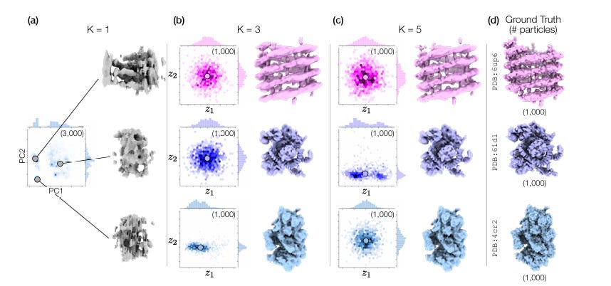
Enter Hydra, from the paper ‘Mixture of Neural Fields for Heterogeneous Reconstruction in Cryo-EM’, published in 2024, where the authors demonstrated exactly that for three structurally different proteins.
How does it work? Really…it’s quite similar to cryoDRGN2. The 5D pose search process is a fair bit more efficient, but a lot of the general concepts are the same. You’re still trying to derive pose information from images via the pose search, after which you feed that and the image into a model that reconstructs a 3D structure, reproject that to 2D via the pose information, and compare the true 2D pose to the predicted 2D pose. So, we can capture conformational heterogeneity and have ab initio reconstruction right out of the box.
How do we deal with compositional heterogeneity? Pretty simple: instead of a single model handling 3D reconstruction, there are now K models (referred to as a neural field in the paper, but, really, it’s just a formal name for the same model as before that intakes in 2D particle images + poses and outputs a 3D structure), where K is equivalent to the number of structures that exist in your cryo-EM dataset. Each model specializes in learning one type of protein structure. How do we decide which model gets which protein? We don’t! When a 2D particle image comes in, all K models try to explain it and we learn which model explains it best, while also figuring out the pose and conformational state. All of the K models are connected in the loss function, so they’ll naturally learn to specialize in a specific protein class (admittedly, I’m skipping over a bit of confusing math here regarding how they are connected...take a look at section 3.3 for more details). At inference time, we simply go with the prediction of the model that seems to explain a given particle the best.
How do we pick K if we don’t actually know how many proteins are in our solution? It’s not heavily discussed in the paper, but the authors do imply that oversized K’s work fine, and undersized K’s look clearly off. In a three protein problem, K’s of 1 failed, K’s of 3 worked, and K’s of 5 had 2 models that no particle ever had high negative log likelihood for. So…just mess with K until you get something reasonable. Who knows how well this scales, hopefully someone discusses that in a future paper.
Again, compositional heterogeneity isn’t really ever exploited! Typical cryo-EM workflow has evolved to actively avoid dealing with it. It’s super interesting that ML has, in this area, somewhat outpaced what the wet lab techniques are actually capable of doing. And to be clear, it intuitively feels like physically preparing a compositionally heterogenous sample is hard; you’d have to deal with potential aggregation, protein-protein interaction, and cause uneven distribution of proteins in the vitreous ice. The future will tell us how hard scaling here is!
What’s left?
In this piece, I’ve primarily walked through how machine learning is changing cryo-EM reconstruction. But there’s still so much that I didn’t explore. Just last month, there was a paper applying ML to the preferred orientation problem. There’s also ongoing work trying to derive molecular dynamics information from cryo-EM maps. I also stumbled across this paper that is trying to use ML to reduce necessary concentrations of purified proteins in cryo-EM by making the particle picking process even better. It goes on from there, in basically every step of the sample preparation process I discussed above, there is someone throwing machine learning at the problem. Jury is still out on how valuable that is, but still!
And, even amongst the methods I’ve written about here, there is still work left to do! Cryo-EM reconstruction is still very much in the early days w.r.t these newer tools; partially due to the relative hesitance of structural biologists of modifying pre-existing workflows, and partially because methods like cryoDRGN2 still have plenty of kinks left to be worked out.
Do we expect structural models like Alphafold to be able to replace the role of cryo-EM anytime soon? As with pretty much all existing wet lab techniques, it is unlikely. The determination of ultra-large protein complexes (which cryo-EM excels at) via pure computational methods is still in a hazy place circa 2024, though of course it may improve with time.
And, ultimately, structural data is important for these models to work at all. The growth of the PDB was something done over decades, painstakingly curated by thousands of scientists. While many view the Protein Data Bank as largely exhausted in utility — a form of fossil fuel that allowed for the creation of Alphafold2 — there may still be room for it to grow massively overnight. Compositional heterogeneity in cryo-EM feels like a brand new way of thinking about structure determination, something that may allow for us to simultaneously characterize tens, hundreds, perhaps thousands of proteins all in one experiment. Is there a world in which we could double the size of the sum total of structural data in a single year? Perhaps. And if there is, it feels deeply likely that cryo-EM, and the machine learning driving its future, will play a role in that.
That’s it, thank you for reading!
- ^
When cryo-EM first came onto the scene, it had to use liquid ethane for cooling, which is kinda a pain to handle. Liquid nitrogen, which is more preferable to work, is not capable of cooling samples fast enough. Why not? People originally thought it was because of the Leidenfrost effect! The nitrogen would produce insulating layer of nitrogen gas around samples dropped into it, which slows down the cooling, giving water molecules enough time to form the aformentioned crystals.
But a study circa 2021 challenges this; they assert that the issue with liquid nitrogen has little to do with the Leidenfrost effect, the problem has to do with there being a thick layer of cold gas thats sits atop liquid nitrogen that pre-cools samples before they hit the liquid! With liquid ethane, this gas layer is simply thinner in size. Once they removed the gas layers from both, they found that they perform roughly the same.
So…why do people still use liquid ethane? The best answer I could find is that experimental determination people have an incredibly hard job, and will not easily switch over to new methodologies unless it’s quite easy. And the existing toolset works well, so why switch?
- ^
The common answer is that copper is meant for structural support of the overlaid carbon film, which is quite flimsy. But then there’s an even more obvious question: why can’t we just abandon the carbon film entirely and just go with copper grids with even smaller holes? Well……I’m not sure. If someone knows the answer to this, reach out to me! I’ll update the post with the answer if I find it.
Edit: Answered! Turns out this grid-of-grid system with the exact same material exists already, such as UltrAuFoil and HexAufoils, though it’s gold instead of copper.
0 comments
Comments sorted by top scores.
