Exploring the Residual Stream of Transformers for Mechanistic Interpretability — Explained

post by Zeping Yu · 2023-12-26T00:36:50.326Z · LW · GW · 1 comments

Contents

  Background: Residual Stream Studies on Attention Layers
  Background: Residual Stream Studies on FFN Layers
  Motivation of Our Research
  Residual Stream
  Distribution Change of Residual Connections
  Contribution Score Designing
  How previous layers/subvalues activate upper FFN layers/subvalues?
  Experiments
    Locating helpful FFN subvalues
    Layer exploration
    Subvalue exploration
    Cross-Layer exploration
  Case Study: “The capital of France is” -> “Paris”
    "Paris” and “London”: analysis on attention layers
    “Paris” and “Bordeaux”: analysis on FFN layers
    Location of FFN Subvalues as “query” and “value”
None
1 comment

— by Zeping Yu, Dec 24, 2023

In this post, I present the paper “Exploring the Residual Stream of Transformers”. We aim to locate important parameters containing knowledge for next word prediction, and find the mechanism of the model to merge the knowledge into the final embedding.

For sentence “The capital of France is” -> “Paris”, we find the knowledge is stored in both attention layers and FFN layers. Some attention subvalues provide knowledge “Paris is related to France”. Some FFN subvalues provide knowledge “Paris is a capital”, which are mainly activated by attention subvalues related to “capitals/cities”.

Overall, our contributions are as following. First, we explore the distribution change of residual connections in vocabulary space, and find the distribution change is caused by a direct addition function on before-softmax values. Second, we prove using log probability increase as contribution score could help locate important subvalues. Third, we find attention/FFN subvalues on previous layers are direct “queries” to activate upper FFN subvalues by inner products. Last, we utilize our proposed method on experiments and a case study, which can verify our findings.

Background: Residual Stream Studies on Attention Layers

The residual stream of transformers has been studied in many works and have been proved useful for mechanistic interpretability. The main characteristic of residual stream is: both the attention and MLP layers each “read” their input from the residual stream (by performing a linear projection), and then “write” their result to the residual stream by adding a linear projection back in. (“A Mathematical Framework for Transformer Circuits”)

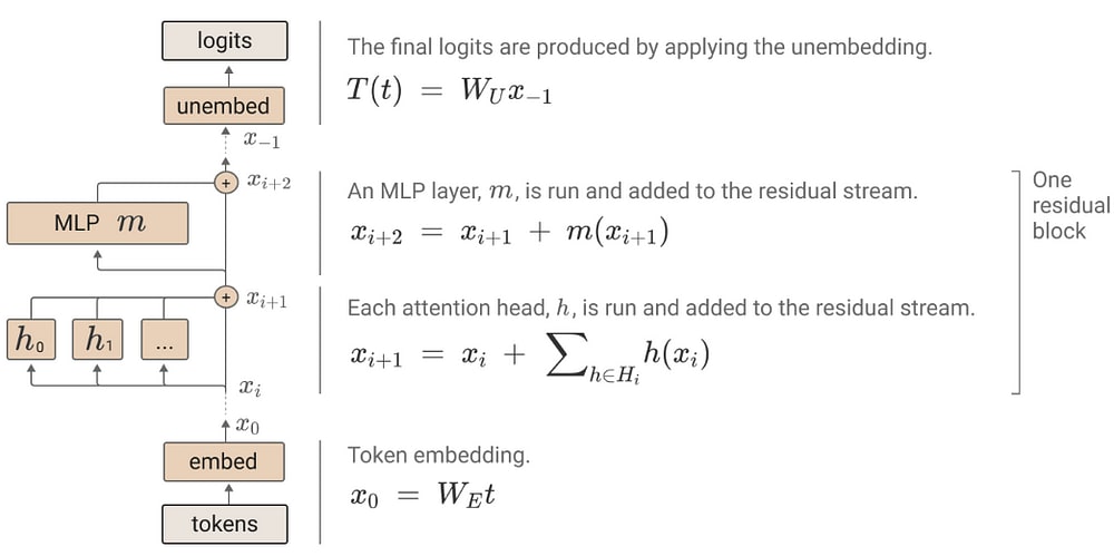
The “A Mathematical Framework for Transformer Circuits” paper focus on attention layers. They build a one-layer attention-only transformer, which can learn skip-trigram relationships like [b] … [a] -> [b] (e.g. [perfect] … [are] -> [perfect]). They also find a two-layer attention-only transformer can learn induction heads like [a][b] … [a] -> [b] (e.g. [Pot] [ters] … [Pot] -> [ters]).

Based on this finding, the “In-context Learning and Induction Heads” paper explore the induction heads. They provide evidence to support the hypothesis: induction heads might constitute the mechanism for the actual majority of all in-context learning in large transformer models.

Background: Residual Stream Studies on FFN Layers

Some other works focus on FFN layers. In the “Transformer Feed-Forward Layers Are Key-Value Memories” paper, the authors find that the FFN layer output of transformer is a direct sum of FFN subvalues. vi is the ith column of the second FFN matrix, and the coefficient score mi is the inner product of input x and the ith row of the first FFN matrix.

                                           

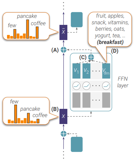
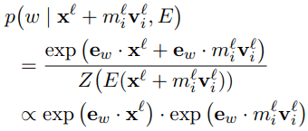
In the “Transformer Feed-Forward Layers Build Predictions by Promoting Concepts in the Vocabulary Space” paper, they find that some FFN subvalues are human-interpretable in vocabulary space. When adding a FFN subvalue mv on x, they believe the probability of word w p(w|x+mv) on vocabulary space is related to the inner products of the word embedding ew and x; ew and mv.

                                                   

Motivation of Our Research

Our first motivation is that we want to explore the distribution change among the whole residual stream including both attention and FFN layers. Most previous work focus on one module (attention/FFN), but in a real model, both attention and FFN layers exist. Furthermore, we aim to explore which layers are more important. For instance, are FFN layers more important than attention layers? Are upper layers more important than lower layers?

Second, we hope to understand the mechanism causing the distribution change, thus we can locate the important subvalues for predicting some token. Even though the previous study find FFN subvalues are interpretable, they haven’t explained how helpful FFN subvalues merge the knowledge into the final prediction, and they haven’t provided the methods to locate the helpful FFN subvalues.

Another characteristic of residual stream is that previous layers and subvalues are direct “queries” to activate upper FFN subvalues. Our third motivation is that we want to design a method to analyze how much previous layers affect upper FFN layers.

Residual Stream

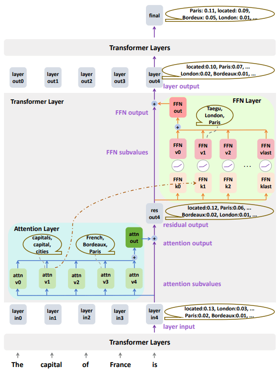
We analyze our work on a 16-layer decoder-only transformer. The layer normalization is added on the input of each transformer layer. There are 4096 subvalues on FFN layers, and the activation function is ReLU. The overall residual stream structure is shown in Figure 1. The layer residual stream is:

                                  

                                                      

where each layer input Lin is the previous layer’s output Lout. Residual output Lres is the sum of layer input and attention output. Layer output is the sum of residual output and FFN output. The attention output and FFN output is also a direct sum computed by a subvalue residual stream:

                                 

Distribution Change of Residual Connections

In layer residual stream and subvalue residual stream, each vector is a direct sum of other vectors (c=a+b rather than c=f(a+b)). Consequently, a key step toward interpreting the mechanism of transformer is to analyze how the distribution of vectors changes between the residual connections.

Let’s rethink the example sentence “The capital of France is” -> “Paris”. In this sentence we hope to explore why the output of the model is “Paris”, so we mainly focus on the probability of word “Paris”. The probability of “Paris” is small in the starting layer input, while it is large in the final layer output. Hence, there must be one or more attention or FFN layers containing helpful knowledge for increasing the probability of “Paris”. Assume the vector before adding is x and the vector with knowledge is v, let’s explore how the probability is increased when adding v on x.

                                  

                                  

                                   

Equations 11–13 show the probability change of word w when vector v is adding to x. Here, w is the word (“Paris”), and the probability of word w is calcaluted by a softmax function among all vocabulary words (assume the vocabulary word number is B), related to the inner products of vector x and word embeddings e1, e2, …, eB.

Let’s term the inner product of ew and x bs-value (before-softmax value) of word w on vector x. Bs-values of all vocabulary tokens are:

                                        

The bs-values have beautiful characteristics. When adding two vectors together, each token’s bs-value is directly added together. And the bs-values corresponds to the probability of words directly.

                                       

From equations 14–16 we can find that when adding a vector v on x, the main thing causing the distribution change is the tokens’ bs-values. The probabilities of tokens with very large bs-values in v will increase.

The “Transformer Feed-Forward Layers Build Predictions by Promoting Concepts in the Vocabulary Space” paper also analyze this distribution change, and they believe the probability of word w is mainly related to the inner products of ew and x, ew and v. However, they forget to take other tokens into account. Here we have some examples to analyze this. Assume there are only 3 tokens in the vocabulary, we focus on the last word’s probability:

(a) bs-value x: [1, 2, 3] -> prob x: [0.09, 0.24, 0.67]

(b) bs-value v: [5, 5, 5] -> bs-value x+v: [6, 7, 8] -> prob x+v: [0.09, 0.24, 0.67]

(c) bs-value v: [1, 1, 1] -> bs-value x+v: [2, 3, 4] -> prob x+v: [0.09, 0.24, 0.67]

Looking at (a), (b), (c), when adding two different vectors with bs-values [5, 5, 5] and [1, 1, 1], the probability of x+v does not change. Therefore, how large a token’s bs-value is not important, while how much larger is more important!

And the distribution change is not only related to the probability of w on v, but also all probabilities on x and v. Thinking about (a), (d), (e), when adding two vectors with same probability on the third token, the distribution change is different.

(d) bs-value v: [1, 4, 5] -> prob v: [0.013, 0.265, 0.721] -> bs-value x+v: [2, 6, 8] -> prob x+v: [0.002, 0.119, 0.878]

(e) bs-value v: [4, 1, 5] -> prob v: [0.265, 0.013, 0.721] -> bs-value x+v: [5, 3, 8] -> prob x+v: [0.047, 0.006, 0.946]

The main finding in this section is that we find the distribution change is caused by a direct addition function on bs-values. When analyzing the outputs of the models, we usually focus on “what are the top words” and “how confident is the model” by looking at the probabilities. The change on probabilities is non-linear. When adding v on x, if we only look at the probabilities on v, we cannot draw the conclusion that tokens with larger probabilities will increase, even though there are some experimental results supporting this. But if we look at the bs-values, we are confident all bs-values on v are added on x directly, thus the probabilities of tokens with large bs-values on v will increase. Also, it is clear to analyze the change of different tokens by bs-values.

Contribution Score Designing

In this section, we explore how to locate the important subvalues for predicting the next word “Paris”. In previous section, we have proved that the mechanism behind the residual connections is a direct sum function on bs-values. Therefore, a helpful subvalue should usually have large bs-values on “Paris”. However, only consider vector v is not enough, since we have explored that the distribution change is related to both v and x. A common method is using the probability increase as contribution score:

                                               Contribution(v) = p(w|x+v) — p(w|x)

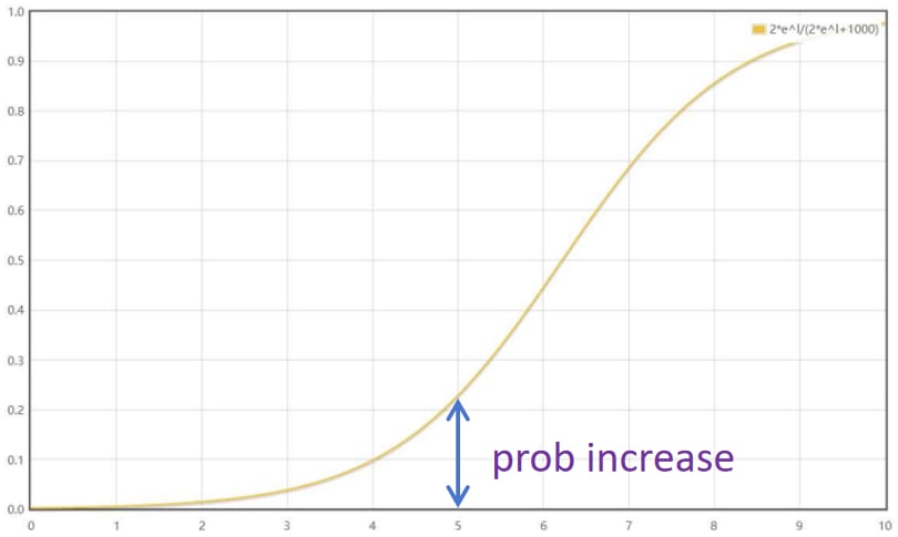
However, in our analysis, using probability increase as contribution score is not fair for lower layers. When adding the same vector, the probability increase is much smaller when adding on a lower layer than adding on an upper layer. The reason of this phenomenon is that the curve of probability increase is not linear. Assume adding a vector v on x:

                                        

The probability of x+v is:

                                            

If we regard exp(bsx) as A, bsv as l, the other denominator term as B:

                                        

The curve of Eq.18 is a non-linear shape:

While the curve of log(F(l)) is more like a linear shape:

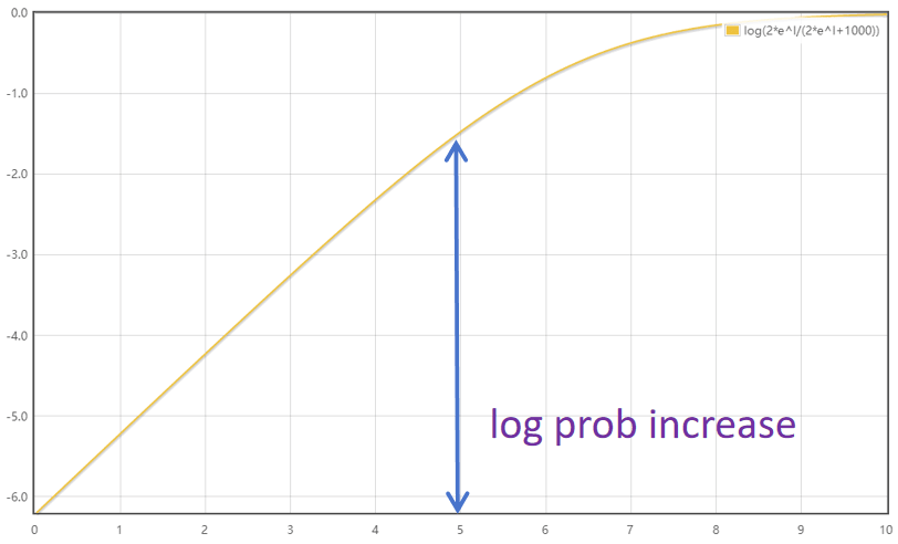
Therefore, compared with probability increase, using log probability increase as contribution score is more reasonable:

                                 Contribution(v) = log(p(w|x+v) )— log(p(w|x))

When computing the layer-level contribution score, v is the attention output or FFN output, and x is the corresponding input of this layer. When computing the subvalue contribution score, v is the attention subvalue or FFN subvalue, and x is still the corresponding input of this layer.

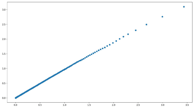
We also explore the relationships of contribution scores on subvalues. The relationships between Contribution(v1+v2) and Contribution(v1)+Contribution(v2) indeedly has a linear monotonically increasing shape (shown in Figure 3), which meets our analysis.

How previous layers/subvalues activate upper FFN layers/subvalues?

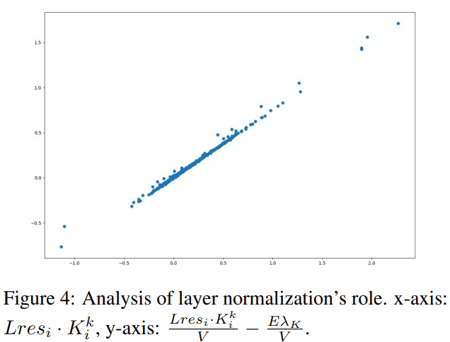
In previous sections, we have analyzed that the model merges a vector’s distribution by adding the bs-values directly. And we can locate important layers and subvalues using log probability increase as contribution scores. In these situations, the subvalues work as “values”. Also, there are subvalues working as “queries” to activate these subvalues. A FFN subvalue is the product of a coefficient score and a fc2 vector (the same in different cases). Therefore, we can see the contribution of “queries” by evaluating how much coefficient scores are activated by the “queries”. But we should first figure out the influence of layer normalization:

                                

                               

                               

The coefficient score is computed by a layernorm input and a vector. Hence, we can compare the inner product of Lres and K (new FFN key), and the sum of first two terms in Eq.23, in order to see how much of coefficient score are affected by layernorm. The relationships are shown in Figure 4.

                                 

The curve is approximately a linear shape. Consequently, we can approximately evaluate the contribution of each previous subvalue/layer-level vector working as “query” to activate one FFN subvalue by computing the inner product between the vector and K (new FFN key). Because Lres is a direct sum of many layer-level vectors (which are also sum of subvalues).

                                      

Experiments

Locating helpful FFN subvalues

We design an experiment to verify our method for locating important subvalues. We randomly sample 1,000 sentences. For each sentence, given the residual output of each layer, we aim to choose 10 FFN subvalues v having the largest probability increase on the predicted token. We compare our method with 3 methods of choosing 10 largest: a) coefficient score, b) product of coefficient score and norm, c) rank of token w. The results are shown in Table 1. Our method achieves the largest score.

                                          

Layer exploration

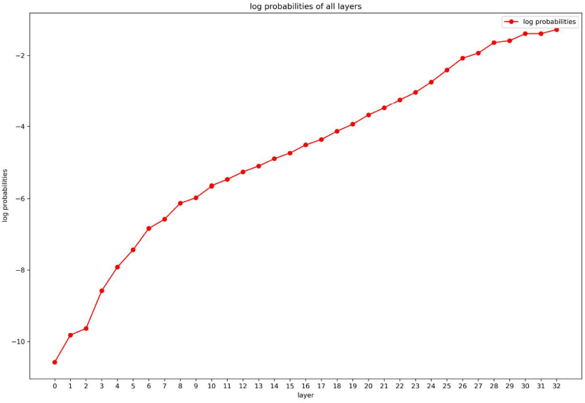
Then we do some exploration on layers and subvalues. First, we want to explore whether there are any layers (lower/upper, attention/FFN) more important than others. So we randomly sample 1,000 sentences and compute the average scores on each layer. The curve is shown in Figure 5. Genearlly, all attention/FFN layers are useful, and all lower/upper layers are useful.

Subvalue exploration

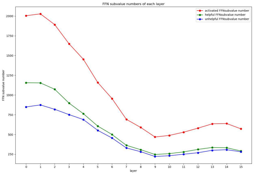
We aim to analyze how many subvalues are helpful for increasing the probability of the final token. The numbers of helpful and unhelpful subvalues are shown in Figure 6. The numbers of both helpful and unhelpful subvalues on lower layers are large than those on upper layers.

We also hope to analyze the proportion of top10 subvalue contribution and all contribution. If this proportion is large, it means contributions are concentrating on a small number of subvalues. On the contrary, it means the contributions are separated. The proportion is shown in Figure 7.

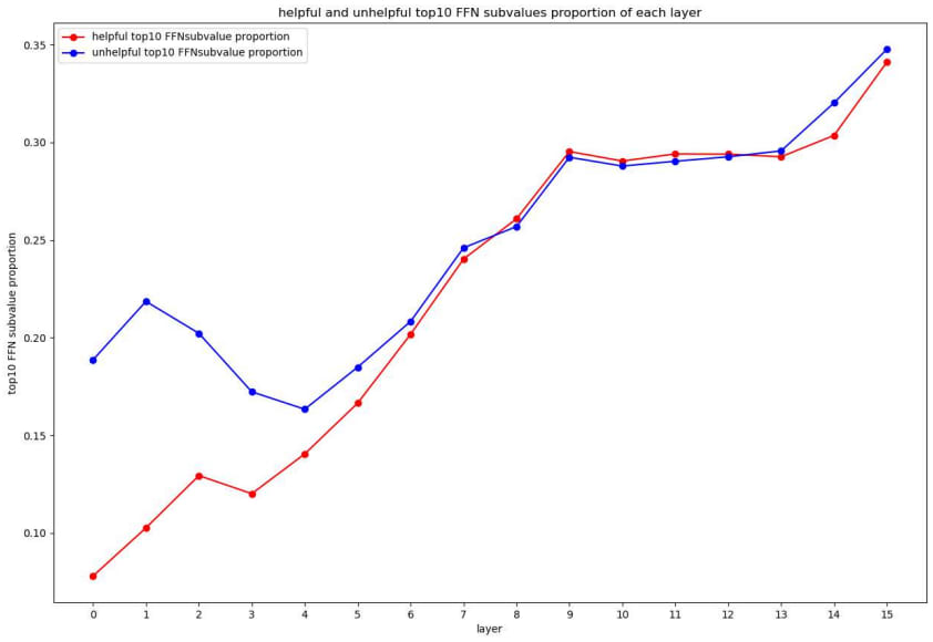
The contributions are more concentrated on upper layers than lower layers, but this may mainly caused by the decrease number curve. Generally, the contributions are separated in various subvalues, because the largest proportion is only 35%.

Cross-Layer exploration

We design a cross-layer score to see how much previous layers affect an upper FFN layer (13th FFN layer in Figure 8). For the upper FFN layer, there are many helpful and unhelpful subvalues. We compute the inner products between previous layer-level vectors and these upper FFN keys, and calculate the sum score of each previous layer. The scores are shown in Figure 8.

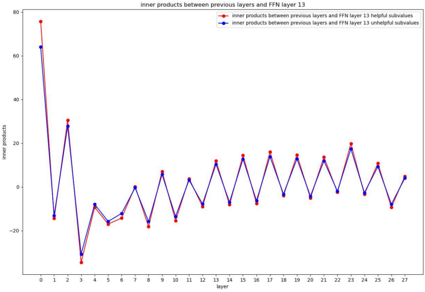
The “zigzag” curve means that attention layers and FFN layers have different ways to affect upper FFN layers. The inner product scores of attention layers are usually larger than 0, so they are more likely to make contribution by enlarging the helpful subvalues’ distributions. On the contrary, the FFN layers are more likely to make contribution by reducing/reversing the unhelpful subvalues’ distributions. Another finding is that all previous layers are playing a role.

Case Study: “The capital of France is” -> “Paris”

At last, we utilize our proposed method on sentence “The capital of France is”. We aim to locate the important parameters in the model for predicting the next word “Paris”. In fact, what we want to explore more is the parameters help distinguish “Paris” from other cities (such as “London”, “Brussels”, “Marseille”, “Bordeaux”). We draw the bs-values of the cities on the residual stream. The results are shown in Figure 9.

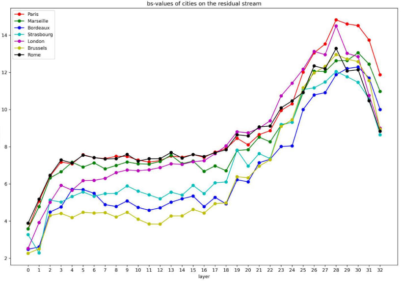
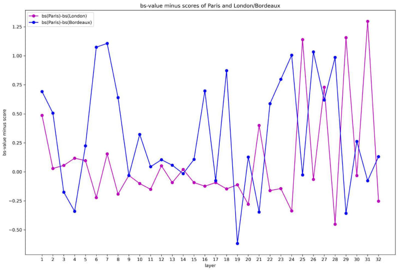
By comparing the bs-values, we can clearly see each token’s bs-value change on each layer. We analyze “London” (another capital) and “Bordeaux” (another city in France). The helpful layers for distinguishing “Paris” and “London” are 12–15 attention layers, while those for distinguishing “Paris” and “Bordeaux” on upper layers are 11–13 FFN layers (see Figure 10).

"Paris” and “London”: analysis on attention layers

We find the helpful subvalues on 12–15 attention layers for distinguishing “Paris” and “London” are all on 4th position, which corresponds to “France”, since they have largest bs-value minus score between “Paris” and “London”. Similar to cross-layer analysis on FFN layers, we hope to design methods to explore which previous layer-level vector plays the largest role. In the first method, we subtract each layer-level vector from the input of attention layer, and recompute the attention subvalues, then calculate the bs-value minus score change between “Paris” and “London”. In the second method, we fix the attention scores and recompute the attention subvalues. The bs-value minus score change of two methods are in Figure 11 and 12.

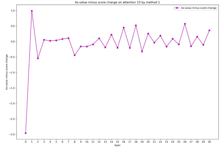
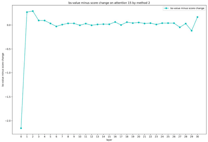
In the first method, almost all previous layer-level vectors affects. In the second method, the embedding of “France” plays a larger role than other layer-level vectors. Therefore, the previous attention and FFN outputs may have an impact on the attention weights more than on attention value vector. Meanwhile, the attention value matrix and output matrix have the ability to extract knowledge “Paris” from word embedding “France”.

“Paris” and “Bordeaux”: analysis on FFN layers

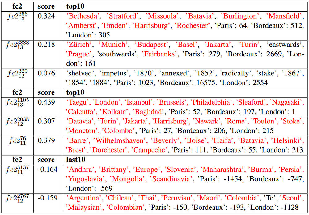
We show the top and last tokens of some 11–13 FFN subvalues in Table 2. In Table 2, “score” means the contribution score for predicting “Paris”. Most helpful subvalues’ top10 vocabulary tokens are related to “city”. In our analysis, most of these subvalues are mainly activated by 9–11 attention layer 2nd subvalue, whose top vocabulary tokens are related to “capitals/cities”. Except helpful subvalues, some unhelpful subvalues’ last10 vocabulary tokens are also related to “city”. Besides, aFFN subvalue with top tokens “18xx” are also helpful for distinguishing “Paris” and “Bordeaux”.

Location of FFN Subvalues as “query” and “value”

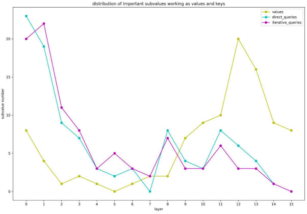
We aim to see the locations of FFN subvalues when working mainly as “value” and “query”. For locating “value”, we utilize the contribution score for predicting word “Paris”. For locating “query”, we design two methods to compute the cross-layer score directly or iteratively. The experimental results are shown in Figure 19. When working as “value”, most high-score subvalues are on upper layers (mainly on the 11 − 13th layer), while working as “query”, subvalues with higher scores are on lower layers (mainly on the 0 − 3th layer).

At last, we conclude the multiple abilities of one FFN subvalue. First, a FFN subvalue can help increase probabilities of tokens with largest bs-values. Second, it can reduce probabilities of tokens with smallest bs-values. Third, it can distinguish two tokens with different bs-values. There are tens of thousands of token pairs in a FFN subvalue, so one FFN subvalue can distinguish many tokens. Last, a FFN subvalue can be a “query” to activate other FFN subvalues. Therefore, if we want to edit one FFN subvalue to update the knowledge in a model, we should be careful and ensure other abilities of this FFN subvalue are not changed.

1 comments

Comments sorted by top scores.