Transformer Dynamics: a neuro-inspired approach to MechInterp
post by guitchounts, jfernando · 2025-02-22T21:33:23.855Z · LW · GW · 0 commentsContents
No comments
How do AI models work? In many ways, we know the answer to this question, because we engineered those models in the first place. But in other, fundamental, ways, we have no idea. Systems with many parts that interact with each other nonlinearly are hard to understand. By “understand” we mean they are hard to predict. And so while the AI community has enjoyed tremendous success in creating highly capable models, we are far behind in actually understanding how they are able to perform complex reasoning (or autoregressive token generation).
The budding field of Mechanistic Interpretability is focused on understanding AI models. One recent approach that has generated a lot of attention is the Sparse Autoencoder (SAE), which hypothesizes that a neural network encodes information about the world with overlapping or superimposed sets of activations; this approach attempts to discover activations inside transformer models that correspond to monosemantic concepts when sparsified or disentangled with the SAE. Work along this path has shown some success—the famous Golden Gate Claude is a great example of an SAE feature corresponding to a monosemantic concept, and one that has causal power over the model (i.e. activating that feature led Claude to behave as if it were the Golden Gate Bridge)—but it also has some limitations. First, in practice, it’s prohibitive to train SAEs for every new LLM; second, SAE features are not always clear or as monosemantic as they should be to have explanatory power; and third, they are not always activated by the feature they are purported to encode, and their activation does not always have causal power over the model.
We were inspired by a trend in neuroscience to focus on the dynamics of neural populations. The emphasis here is both on dynamics and on populations, and the underlying hypothesis is that important neural computations unfold over time, and are spread across a group of relevant neurons. This approach is in contrast to analyses that focus on individual units, and those that treat computation as a static process.
Some notable examples where the population dynamics approach has yielded insights has been in the motor cortex, where preparatory activity before a movement sets the system up for proper initial conditions during movement, and unfolds in a null subspace that’s orthogonal to activity during movement. Moreover, during movement, motor cortex activity appears to show low-dimensional rotational dynamics, which some have proposed to form a basis for muscle commands. Such activity patterns demonstrate attractor-like dynamics, as demonstrated by optogenetic perturbation experiments in which the population jumps back to its trajectory after being offset with an optogenetic stimulus. Attractor-like dynamics have been demonstrated during working memory tasks, too, where decision points have been shown to follow a line attractor.
Unlike the brain, transformers do not follow any explicit temporal computation. However, the residual stream in these models can be thought of as a vector whose activity unfolds over the layers of the model. In transformers, the residual stream is linearly updated twice in every layer: following the attention operations, and following the MLP. For a 32-layer Llama 3.1 8B, this is 64 pseudo-time steps for each token during which the residual stream evolves.
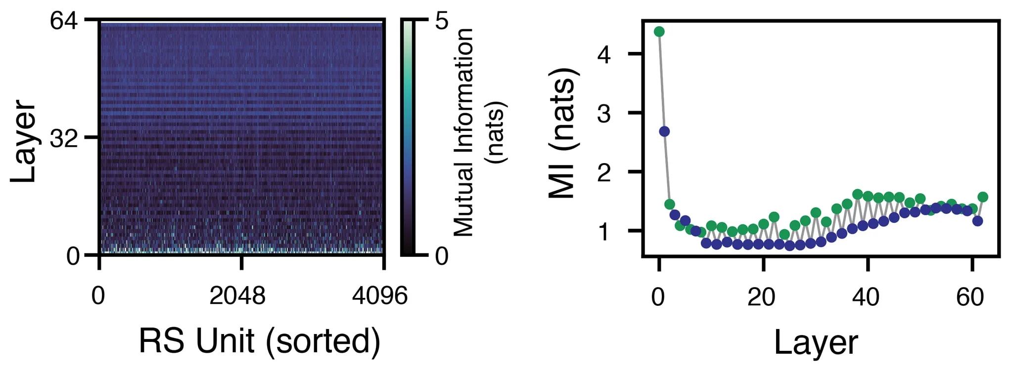
We began this work by simply looking at the activations of the RS. The first interesting finding was that the RS activations increased in density over the layers, with most individual “units” increasing in magnitude. (Since the individual dimensions of the RS are not neurons per se, we refer to them as “units,” in analogy to electrophysiological recordings in the brain, where electrical signals ascribed to individual neurons are termed thus).
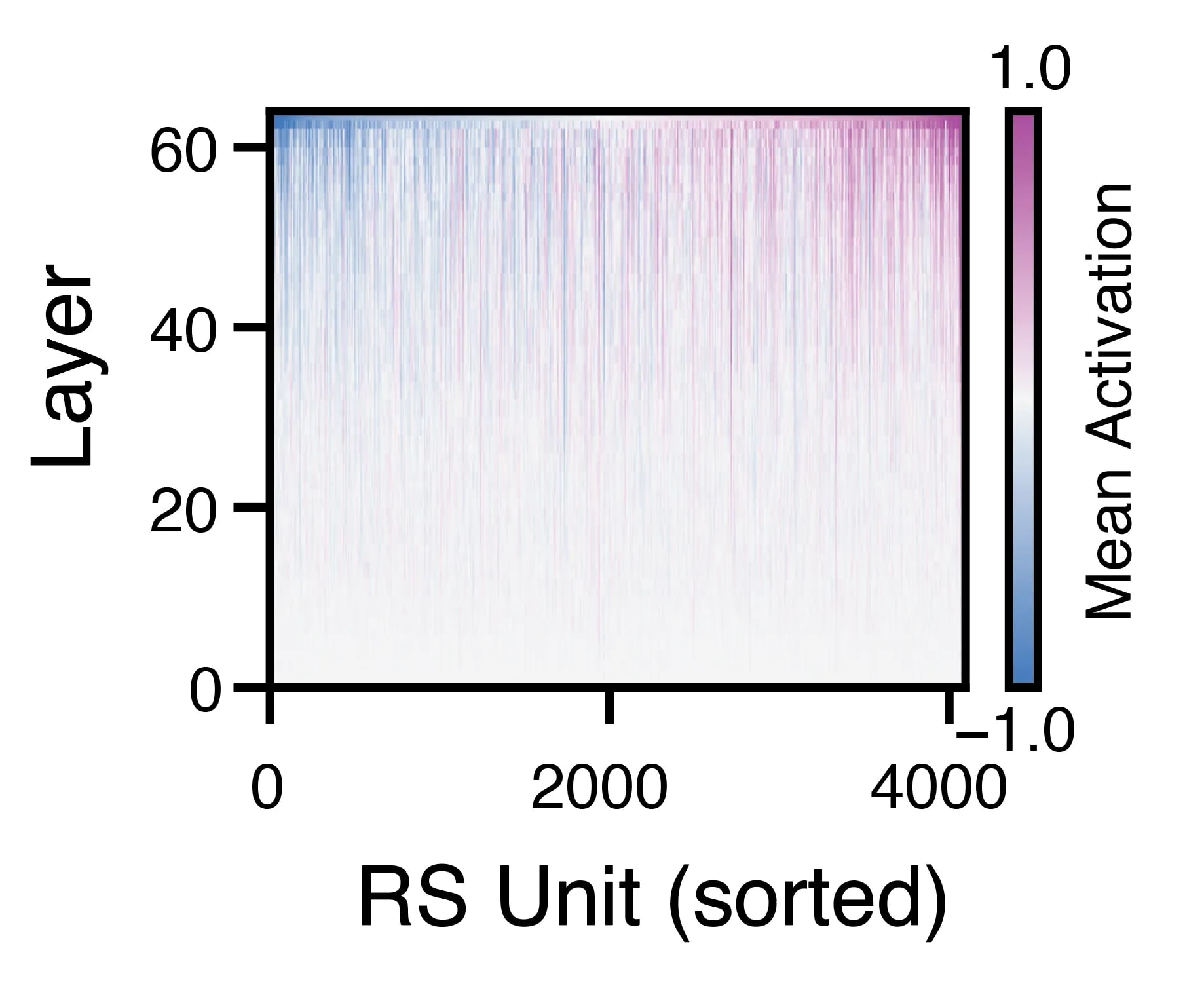
While the lower layers had mostly low-magnitude activations, this sparsity gave way to a dense set of activations in the higher layers. This was surprising because there is no apriori reason for the RS vector to grow like this—it would have been equally as plausible for each attention and MLP block to “write” negative values to subspaces in the RS, and for the whole thing to be stable in magnitude over the layers.
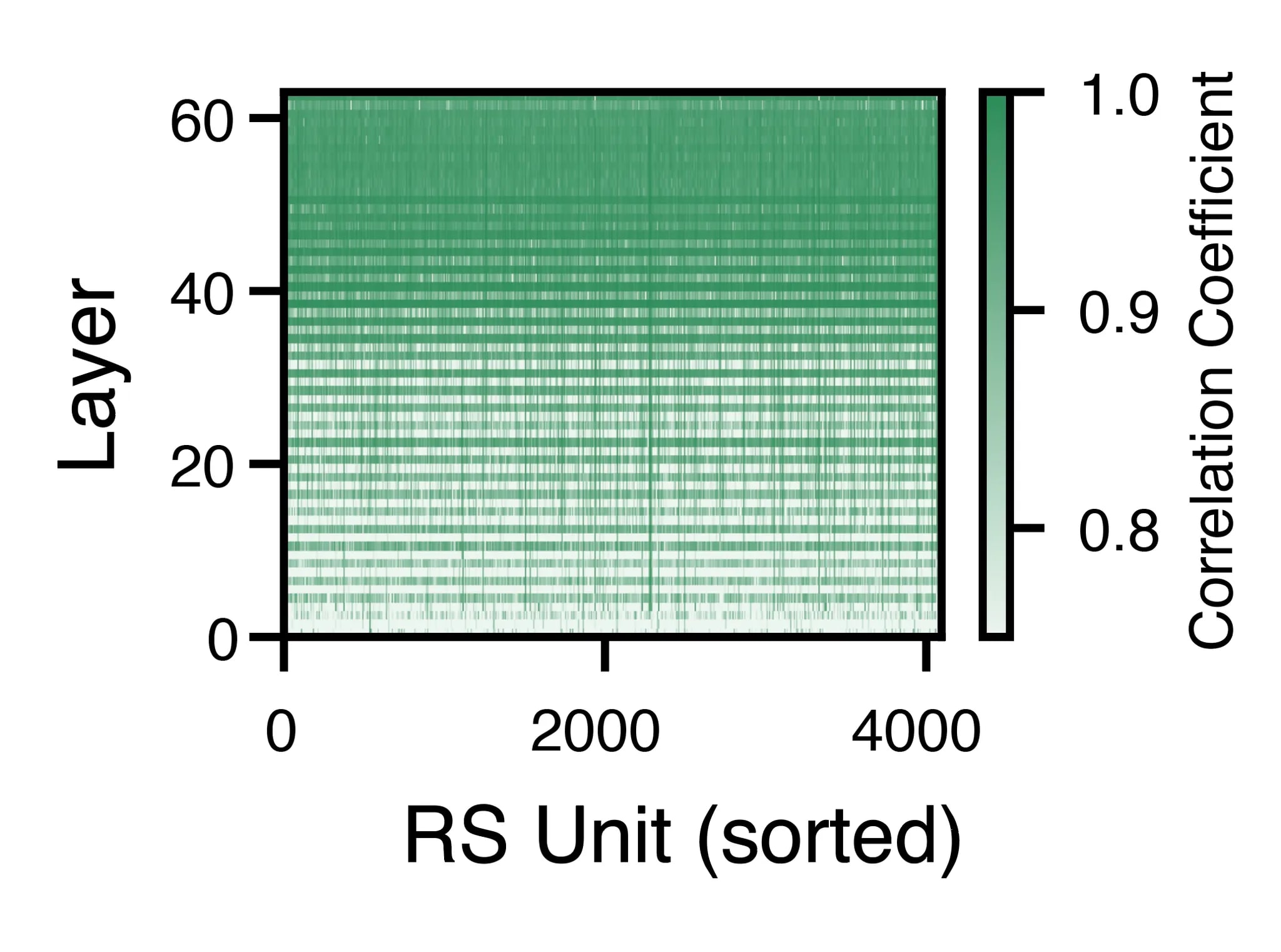
The next surprise was the overall similarity of each unit’s activation on successive layers. For a given unit, its activation over 1000 data samples was highly correlated to its activation on the next layer. These correlations increased over the layers, and were even higher for the attention-to-MLP transition within a layer than for the MLP-to-attention transition across layers.
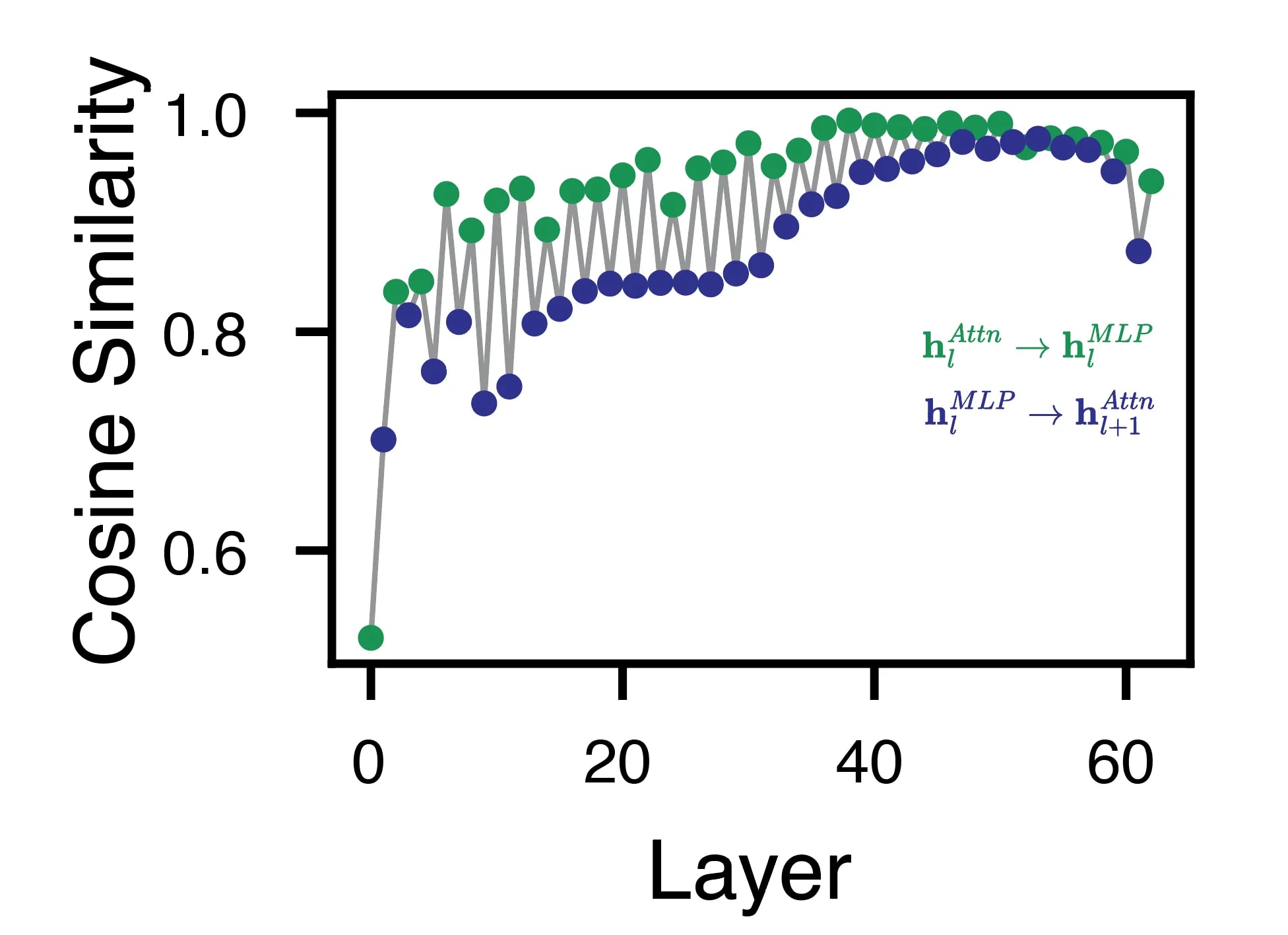
A slightly different perspective on how the RS changed from layer to layer was the cosine similarity of the RS vector from one sublayer to the next. From this whole-vector perspective, the RS grew in similarity over the layers, again with higher similarity for within-layer transitions.
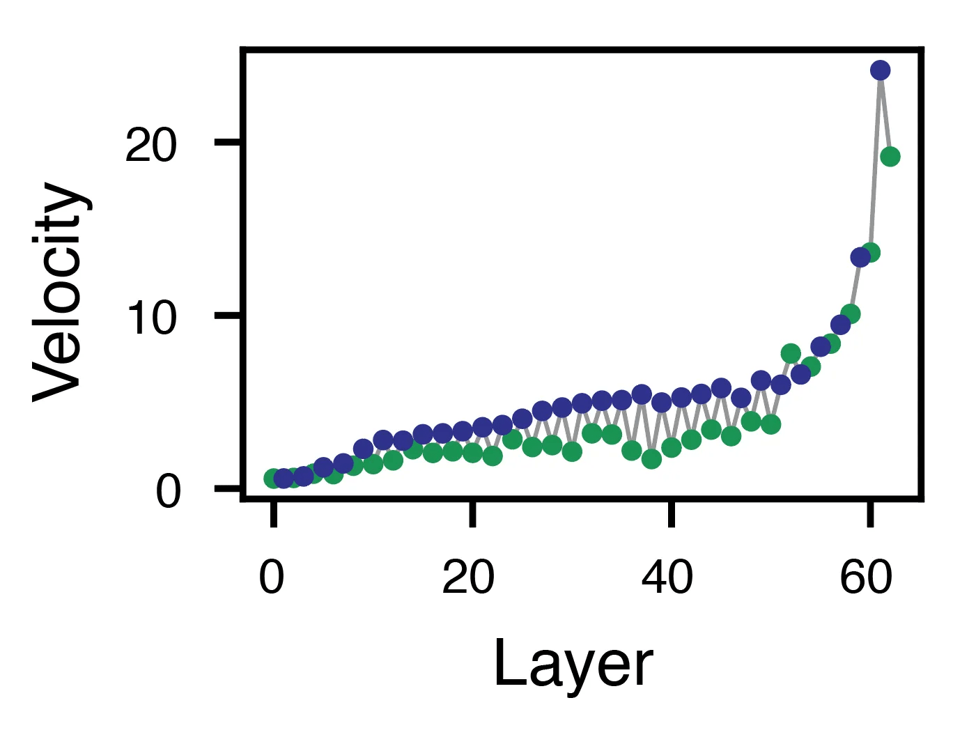
As these vectors grew more and more similar, they also increased in velocity, accelerating from one layer to the next.
Surprisingly, while the cosine similarity started relatively high and grew, mutual information dropped precipitously in the first several steps. It then grew slowly but surely for the cross-layer MLP-to-attention transitions, and a bit more haphazardly for the within-layer attention-to-MLP transitions.
We next wanted to zoom in a little and ask what the individual unit activations looked like, and how they changed over “time” (i.e. layers). Such phase-space portraits revealed rotational dynamics with spiraling trajectories in this activation-gradient space. These tended to spin out over the layers, starting with small circles that increased in magnitude.
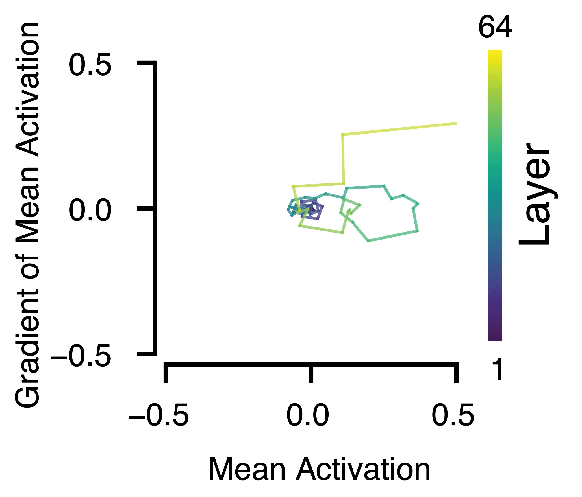
While these weren’t exactly smooth trajectories, they were clearly rotational, sometimes rotating along the origin in this space, and sometimes starting at the origin and then drawing circles about other locations. On average, the RS units circled this space ~10 times over the 64 sublayers (compared to basically zero for units whose layers were shuffled prior to the rotational calculation.
We were keen to see how the dynamics of the RS evolved as a whole. This this end, we trained a deep autoencoder that progressively compressed the representations into a bottleneck down to 2D (we termed this the Compressing Autoencoder (CAE) to highlight the contrast to the expanding Sparse Autoencoder (SAE) approach).
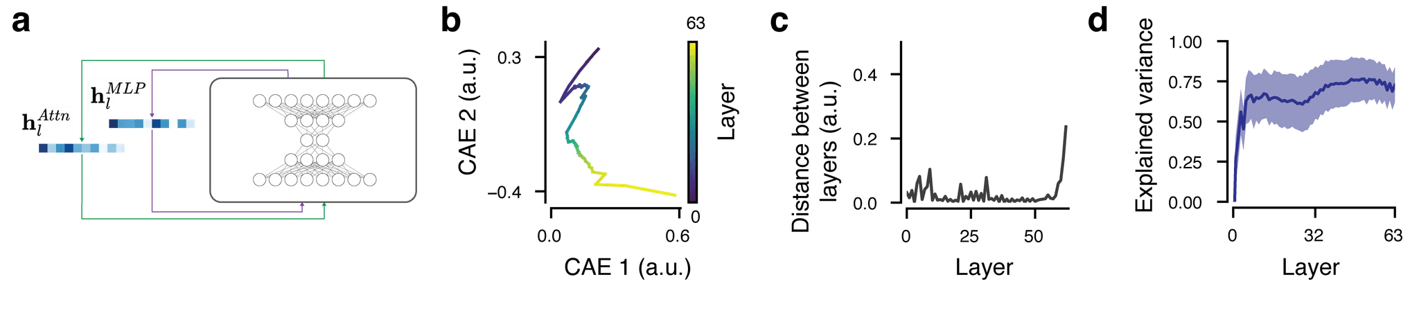
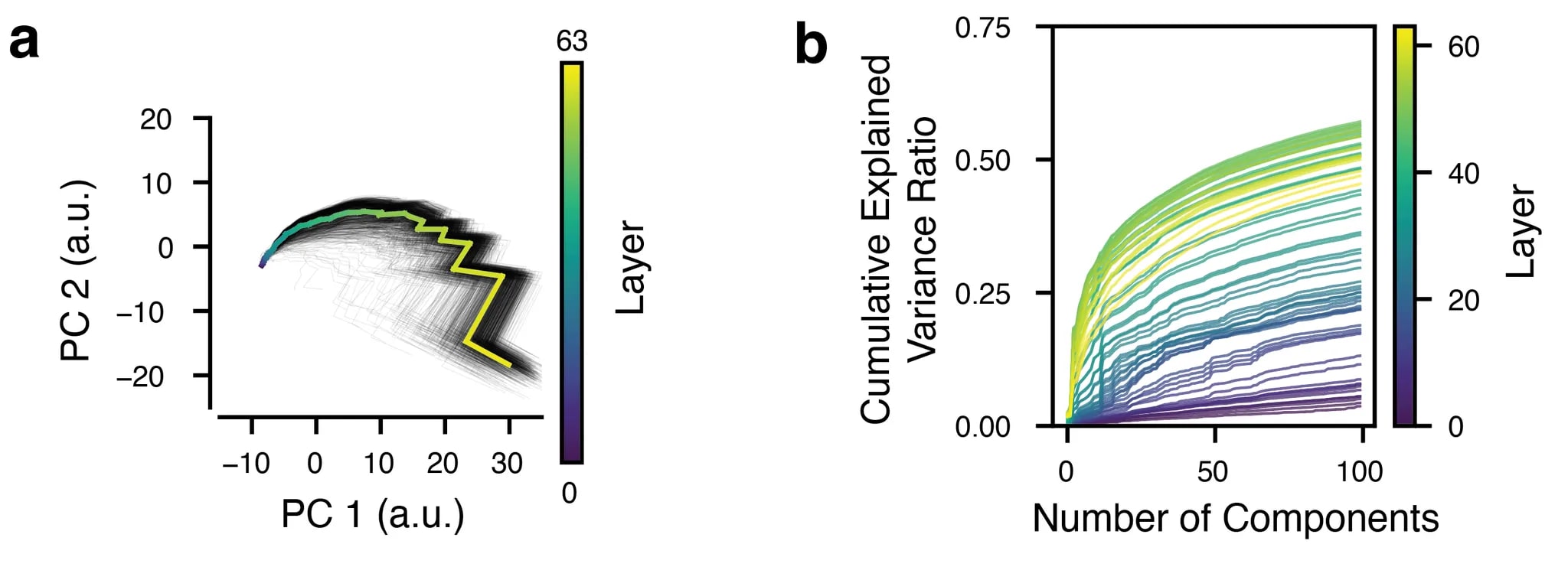
The CAE treated every sublayer’s RS vector as a separate data sample to encode and reconstruct, which opened the window to asking how these vectors evolve over the layers. The dynamics overall were low-dimensional, but the earlier layers were harder to reconstruct than the later ones, the explained variance jumping after the initial few sublayers, leveling out up until halfway through the model, and then slowly increasing again until the end. This was paralleled by representations revealed by PCA, where the lower layers showed higher dimensionality than the later layers.
The PCA was also instrumental for our final experiment here, in which we asked whether the RS exhibits one of the hallmarks of dynamic systems: attractor-like dynamics. To test this, we created a grid of points in the 2D PC space to which we would “teleport” the RS.
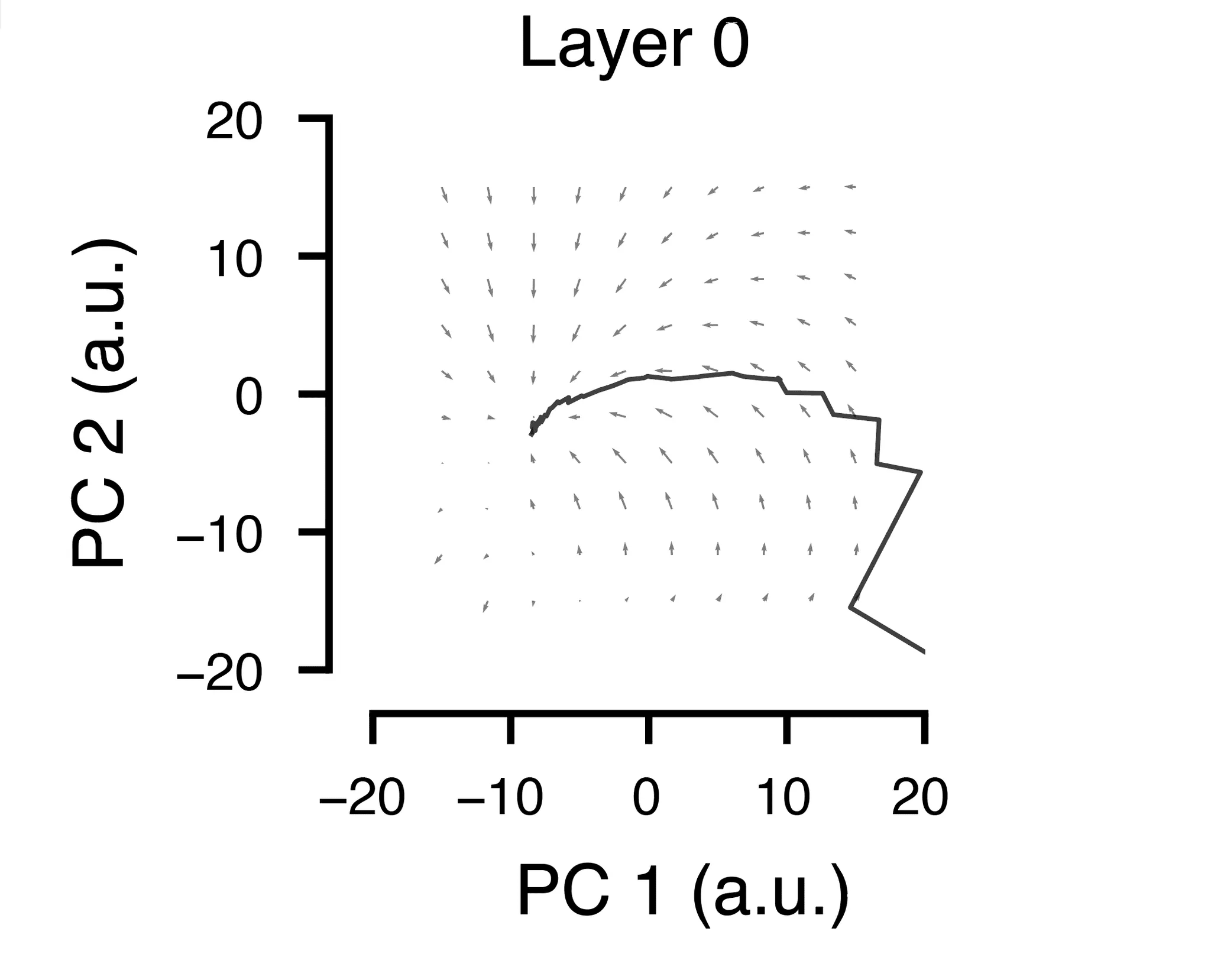
The resulting quiver plots, which show the magnitude and direction of the RS trajectories after teleportation (based on the first 12 sublayers in this case) show an interesting pattern: For most starting positions in this space, the trajectory was pulled toward its “natural” starting place. In reality, since these trajectories don’t unfold over infinite time, the final positions at the end of the 64 sublayers do not return to the normal trajectory. It would be interesting to see if a recurrent model trained on RS vectors can do this, and how it might transform those vectors if allowed to run for many more time steps than 64.
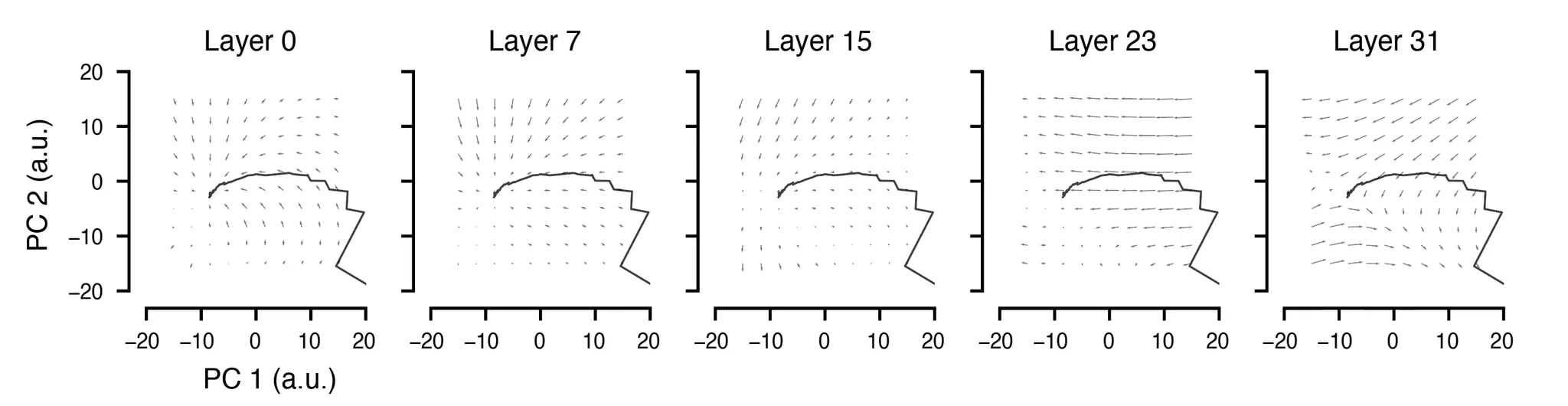
We repeated this experiment for several different layers and note that it’s mostly the earlier layers that exhibit this property of moving the RS back to its original position. Perturbations halfway up the model or later seem to still have coherent flows, but these were not directed toward toward the original positions.
This initial foray into treating the transformer as a dynamical system leaves many questions unanswered. This collaboration was a side project for the both of us, to which we devoted spare time outside of our main work.
Still, we are excited to see where this can go. As AI models grow more powerful, it will be crucial to understand and be able to predict their inner workings, whether for completely closed models (i.e. just an input/output API) or those with various levels of openness. In cases where we have access to weights but not the training data, interpretability tools will serve important roles in reading the AI’s mind in the service of safety.
The neuroscientific inspiration here is threefold:
- Analyzing and visualizing activations and their statistics: yes, others have done a lot of work on visualization the activations of some AI models (e.g. Distill), but the neuro approach arguably has a richer tradition of visualizing and interpreting big, messy data.
- Dynamical systems: while dynamical systems theory is not a neuroscientific concept, it has in the past decade been a
- Neural Coding theory: neuroscientists have spent a long time thinking about how neurons might encode information about the world and perform relevant computations on that information, transforming representations as they propagate from one brain area to another. Some of these approaches have been more successful than others, and our hope is that MechInterp can benefit from the the more promising ideas.
The paper: https://arxiv.org/abs/2502.12131
0 comments
Comments sorted by top scores.