In Most Markets, Lower Risk Means Higher Reward

post by dawangy · 2021-08-13T17:32:16.585Z · LW · GW · 13 comments

The age old adage that high risk is associated with high expected return has not been true in the U.S. stock market, at least when using the academic standard of measuring risk with the either beta or standard deviation of returns. This claim is one of plain numbers, so by itself, it is not disputed. However, the reasons for the existence of this phenomenon, as well as its practical exploitability are. Here we will explore different hypotheses about why this is the case, including some hypotheses that are consistent with the EMH and some that are not.

In my view, the most comprehensive empirical study of a similar result was in Frazzini and Pedersen. In this paper the authors examined the low beta phenomenon by constructing hypothetical portfolios that are long low beta stocks and short high beta stocks in market-neutral ratios. Using this approach, the authors determined that low beta was associated with excess returns in 19 out of 20 countries' stocks, and was also true in many alternative markets such as those for corporate bonds, treasuries, foreign exchange, and commodities. The in-sample effect was strongest in the Canadian stock market, and the Austrian stock market was the only studied market for which the effect was (very slightly) negative. The out of sample construction based on the methodology created in sample was also positive in all nations studied except Sweden. Note that this is slightly different from my headline, as it suggests that the "risk-adjusted" returns of low beta stocks is higher than those of high beta stocks. Not necessarily that the returns of low beta stocks are higher in general.

The hypothesis of Frazzini and Pedersen is that some investors are leverage constrained, meaning that they are less capable of borrowing funds in order to increase exposure to equity. This leads those less capable of leverage to seek the higher expected returns dictated by their preferences through exposure to riskier stocks, which reduces the risk adjusted expected returns of riskier stocks because investors will purchase them at discounted expected returns to achieve artificial market leverage. The paper illustrates that under the framework of modern portfolio theory, it is mathematically true that certain kinds of investors that they describe will yield the types of results they are describing.

Since it was written by researchers working at AQR, its almost certainly true that the authors believe that the factor is exploitable. Otherwise, it wouldn't be a great advertisement for their collection of low beta mutual funds. For what it's worth, those funds are some of the only equity funds they offer that have actually generated alpha in their lifetime. Most haven't. The CEO of AQR claims he is "in the middle" in terms of his belief in the EMH, but to be honest his words and actions sound more to me like he doesn't believe in it.

In response, Novy-Marx and Velokov dispute the idea that the low beta factor violates the EMH by suggesting that 

1. A value weighted version of the factor is closer to what investors can reasonably exploit in practice because firms with very low capitalization are very illiquid and can't be readily turned over without incurring significant costs. This value weighted version shows a lower excess return.
2. The most recent additions to the Fama-French 5 factor model (explained later)  explain the bulk of the effect, and the remaining outperformance is not significant. In their words, low beta "earns most of these returns by tilting strongly to profitability and investment... The strategy’s alpha relative to the Fama and French five-factor model is only 24 bps/month, and insignificant (t-statistic of 1.63)."

The Fama-French Factor Model is probably the most academically accepted model of excess market returns, and is often used in defense of the weak EMH. It tries to explain that some stocks have variation in risk adjusted returns, but only because there are other risks at the level of each company's fundamentals for which investors are compensated for taking on. For example, it posits that investing in small companies has inherent risks that may not be reflected in price volatility, and so therefore investors who invest in smaller firms will receive higher risk adjusted returns for taking on this risk.  "Profitability and investment" mentioned in the last section are the names of two such risk factors added to the Fama-French model in 2013/2014 and published in 2015.

Where do I stand on this issue? Well to be honest I have personal issues with both of the explanations presented. Perhaps it is because I'm not a real researcher like these people and misunderstand what they're saying. Nevertheless, I'll start by airing my complaints about Frazzini and Pedersen. Their hypothesis that leverage constrained investors choose instead to invest in higher beta due to rational optimization seems suspect to me because in the U.S., stocks with higher beta or volatility do not even have higher absolute returns without adjusting for risk.

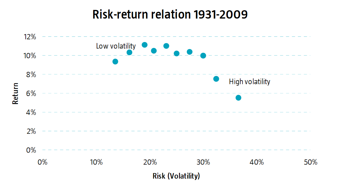
Admittedly, this chart isn't from a purely academic source, but the strength of the prior evidence is convincing enough that I believe what the authors are saying. Why would leveraged restricted rational investors try to get higher expected returns by tilting their portfolios to stocks that are probably just worse?

I also don't like the counter-explanation by academics like Novy-Marx (but also some others) that the low beta phenomenon is explained by the latest two factors in the Fama-French Model. Originally the Fama-French model only had 3 fundamental risk factors. If things don't quite work out after the first 3, it seems awfully ad-hoc to just find 2 more and then add them to the back. There also seems to be a belief in academia that getting higher risk adjusted returns through analysis of company fundamentals is more possible than getting them through historical price data. After all, the "weak" form of the EMH states that it is possible to get higher risk adjusted returns through fundamental analysis but not historical price analysis, while the "semi-strong" form states that it is not possible through either fundamental or price analysis, and only possible for those with material nonpublic information. Why isn't there a version of the EMH that states it is only possible through analysis of price history and not through company fundamentals? (For the record, I don't believe this.) 

The people who trade actively in industry know that quantitative investors do use price history in making decisions. "Trend following" is one of the most popular CTA strategies and it means exactly what it sounds like, i.e. "buy what went up recently." These trend followers have produced alpha, although markedly less in recent years. Perhaps it is a bit unfair to include high frequency traders into the mix, but they obviously qualify too.  So then, if price history is useful according to those in industry who are undoubtedly successful in more ways than just luck (like D.E. Shaw, Citadel, RenTech, etc.), why force the conversation back into fundamental risk factors (and two that seem very arbitrary, at that)?

The low volatility phenomenon remains a mystery to me, and I don't find satisfaction in reading results from academia that try to explain its existence.

13 comments

Comments sorted by top scores.