Making better estimates with scarce information

post by Stan Pinsent (stan-pinsent) · 2023-03-22T17:40:55.318Z · LW · GW · 5 comments

Contents

  TL;DR
  Summary
  Interval vs point estimates
    Core examples
    Point estimates are fine for multiplication, lossy for division
    Interval estimates are prone to bias
    General findings: interval vs point estimates
  Normal vs Lognormal modelling
    A high ratio between interval bounds implies positive skew
    General findings: normal vs lognormal
  Creating aggregate estimates
    The geometric mean is usually better than the arithmetic mean
    Weighted means
    General findings: aggregate estimates
  Conclusion: complexity vs legibility
      Changes
None
5 comments

TL;DR

I explore the pros and cons of different approaches to estimation. In general I find that:

• interval estimates are stronger than point estimates
• the lognormal distribution is better for modelling unknowns than the normal distribution
• the geometric mean is better than the arithmetic mean for building aggregate estimates

These differences are only significant in situations of high uncertainty, characterised by a high ratio between confidence interval bounds. Otherwise, simpler approaches (point estimates & the arithmetic mean) are fine.

Summary

I am chiefly interested in how we can make better estimates from very limited evidence. Estimation strategies are key to sanity-checks [EA · GW], cost-effectiveness analyses and forecasting.

Speed and accuracy are important considerations when estimating, but so is legibility; we want our work to be easy to understand. This post explores which approaches are more accurate and when the increase in accuracy justifies the increase in complexity.

My key findings are:

• Interval (or distribution) estimates are more accurate than point estimates because they capture more information. When dividing by an unknown of high variability (high ratio between confidence interval bounds) point estimates are significantly worse.

 

• It is typically better to model distributions as lognormal rather than normal. Both are similar in situations with low variability, but lognormal appears to better describe situations of high variability..

 

• The geometric mean is best for building aggregate estimates. It captures the positive skew typical of more variable distributions.

 

• In general, simple methods are fine while you are estimating quantities with low variability. The increased complexity of modelling distributions and using geometric means is only worthwhile when the unknown values are highly variable.

Interval vs point estimates

In this section we will find that for calculations involving division, interval estimates are more accurate than point estimates. The difference is most stark in situations of high uncertainty.

Interval estimates, for which we give an interval within which we estimate the unknown value lies, capture more information than a point estimate (which is simply what we estimate the value to be). Interval estimates often include the probability that the value lies within our interval (confidence intervals) and sometimes specify the shape of the underlying distribution. In this post I treat interval estimates as distribution estimates as the same thing.

Here I attempt to answer the following question: how much more accurate are interval estimates and when is the increased complexity worthwhile?

Core examples

I will explore this through two examples which I will return to later in the post.

Fuel Cost: The amount I will spend on fuel on my road trip in Florida next month. The abundance of information I have about fuel prices, the efficiency of my car and the length of my trip means I can use narrow confidence intervals to build an estimate.

Inhabitable Planets: The number of planets in our galaxy with conditions that could harbour intelligent life. The lack of available information means I will use very wide confidence intervals.

Point estimates are fine for multiplication, lossy for division

Let’s start with Fuel Cost. Using Squiggle (which uses lognormal distributions by default; see the next section for more on why), I enter 90% confidence intervals to build distributions for fuel cost per mile (USD per mile) and distance of my trip (miles). This gives me an expected fuel cost of 49.18USD

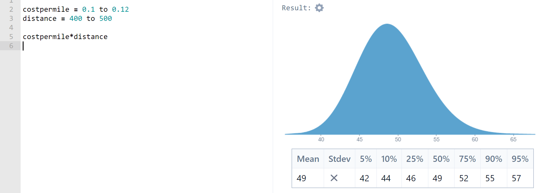
What if I had used point estimates? I can check this by performing the same calculation using the expected values of each of the distributions formed by my interval estimates.

I get the same answer. In fact, this applies in all cases: if X and Y are normally or lognormally distributed,

$$E\left(X\right)E\left(Y\right)=E\left(XY\right)$$

In other words, the mean of the product of two normal/lognormal distributions is the product of their means. The only drawback of using point-estimates for multiplication is that you only get a numerical answer - you lose the shape of the distribution.

What about division? Put simply, 

$$E\left(1/Y\right)\ne 1/E\left(Y\right)$$

so 

$$E\left(X/Y\right)\ne E\left(X\right)/E\left(Y\right)$$

Division will be lossy when you use point estimates. But how bad is it?

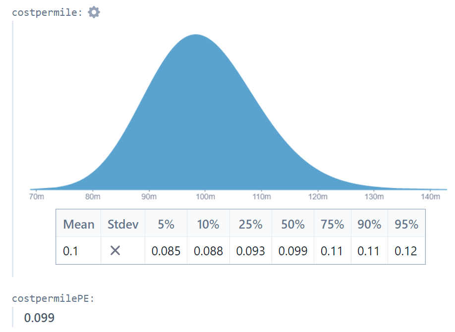
Using the Fuel Cost example we find that the point estimate result (0.099048) is within 1% of the interval estimate result (0.099809).

Now let’s turn to the inhabitable planets example. I use interval estimates for the number of stars in the galaxy and the number of stars per inhabitable planet. Because of the uncertainty the bounds of my intervals differ by 2-3 orders of magnitude.

 

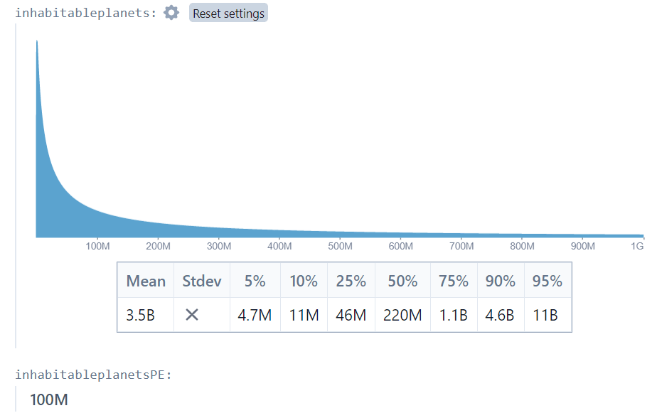
I find that the interval-estimate approach gives an expected number of inhabitable planets of 3.5 billion, while my point-estimate approximation is just 100 million! Clearly when there are very high levels of uncertainty, dividing by a point estimate is inaccurate. Not only that, but the point estimate answer provides no information on the shape of the possible outcomes. The interval estimate approach shows us that although the expected number of planets is 3.5 billion, the median is just 220 million. 

This heavy-tailed behaviour helps explain where the Drake Equation (which relies upon point-estimates of highly uncertain values and suggests that we should have heard from aliens by now) goes wrong: using interval estimates we can show that although the expected number of interstellar alien neighbours is high, the median is much lower. My very rough attempt finds a mean of 4700 alien neighbours, with a a 25-50% chance of none at all (although I may be pushing Squiggle past its limits).

Interval estimates are prone to bias

Interval estimates are excellent for back-of-envelope Fermi problems. But it is difficult to build them in an objective way. Suppose I have several point-estimates for the fuel efficiency of my car - I can easily take a weighted average of these to make an aggregate point estimate, but it’s not clear how I could turn them into an interval estimate without a heavy dose of personal bias. I may return to this problem in the future, but for now I consider interval estimates to be best for rough, unaccountable, Fermi [EA · GW]-style calculations or for situations where the underlying distribution is well understood.

General findings: interval vs point estimates

I did some more experimentation on Squiggle to generalise the findings slightly.

• It's OK to multiply point-estimates. They will give the same mean as the mean of the product of two distributions.
• Dividing by a point-estimate is accurate when the ratio between the interval bounds is low, and performs poorly when the ratio is more than 2. For example:
  • When dividing by a (lognormal, 90% C.I.) distribution where the upper bounds are 1.2 times the lower bounds, the point-estimate approach underestimates by 0.3%
  • When dividing by a (lognormal, 90% C.I.) distribution where the upper bounds are 2 times the lower bounds, the point-estimate approach underestimates by 4.3%
  • When dividing by a (lognormal, 90% C.I.) distribution where the upper bounds are 10 times the lower bounds, the point-estimate approach underestimates by 39%
• Interval estimates are prone to personal bias. It’s easy to create an interval estimate intuitively. When objectivity is important and the evidence base is sparse, point estimates are easier to form and are more transparent.

Normal vs Lognormal modelling

Squiggle uses lognormal distributions by default. Why?

In this section we will find that lognormal distributions are very similar to normal distributions when they share the same, narrow confidence intervals. As the intervals widen the distributions diverge, and the lognormal distribution usually becomes superior. Hence I suggest that using the lognormal distribution by default is the best strategy. I don't consider other distributions (like the power-law distribution) that may be an ever better fit in some cases.

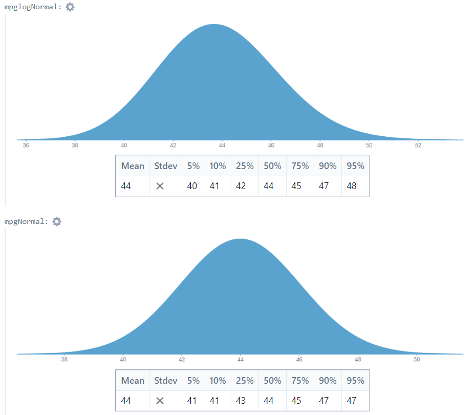
Turning to the Fuel Price example, we see that the normal/lognormal choice makes little difference when the ratio between interval bounds is small:

In this case lognormal and normal look very similar, and the distributions give means of 39.885 and 40 respectively.

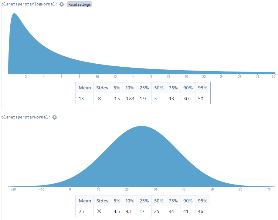
With the Inhabited Planets example, however, there is a different story. Using 0.5 and 50 as the 5th and 95th percentiles, I get very different-looking distributions:

The means are 13.32 and 25.25 for the lognormal and normal models respectively, and the shapes are very different.

Which is a better match for our understanding of the situation? In my opinion, the lognormal distribution is better. if we expect the number of planets per star to be between 0.5 and 50, the “expected” number of planets should be closer to 13 than to 25. Furthermore, the normal distribution assigns a nontrivial probability to (impossible) negative outcomes.

I think it’s clear that in this case the lognormal distribution is superior. But that’s just a gut feeling. Let’s explore this.

A high ratio between interval bounds implies positive skew

Consider datasets with a high ratio between the 5th and 95th percentiles:

• The lengths of rivers (often used to exemplify Benford’s law)
• The populations of cities/countries
• Property prices

These all have positively-skewed distributions that could be approximated by the lognormal distribution.

Now consider broadly symmetric datasets:

• The heights of adult males
• The durations of pop singles
• The price of gas in Florida gas stations today

These could probably be modelled with the normal distribution. Notice that in all of these cases, the ratio between the 5th and 95th percentiles will be low. A tall man is perhaps only 20% taller than a short man.

So in general a high ratio between 90% C.I. bounds implies positive skew and is hence better modelled by a lognormal distribution.

This isn’t a rigorous argument, but I suspect that you will struggle to think of examples that buck the trend. I can think of one. It’s possible that a normally-distributed variable could happen to have a small, positive 5th percentile. This would lead to a high ratio between 5th and 95th percentiles: suppose the temperature in my hometown has 5th and 95th percentiles of 0.1°C and 30.0°C respectively. The ratio between the bounds is 300, but the underlying distribution is probably symmetric and best modelled by a normal distribution. Note that the rule of thumb would apply if we measured temperature in Kelvin instead.

General findings: normal vs lognormal

• The lognormal and normal distributions are similar when the ratio between interval bounds is low. The difference in means is just 3.6% when one bound is 2x the other.
• The lognormal distribution is usually superior when the ratio between interval bounds is high. These circumstances usually imply negative skew, which make the lognormal distribution a better fit.
• Although the lognormal is usually better, there are important considerations:
  • The lognormal distribution can only model positive values.
  • If you have reliable estimates of the mean and/or standard deviation of a distribution, the normal can be easier to model with.
  • Quantities with strict upper bounds (such as probabilities) may not be suitable for the lognormal distribution, although the normal distribution is usually not suitable either in these instances.
  • Not everything is positively-skewed or symmetric. The number of teeth in the next dental patient’s mouth, for example, would likely be positively skewed. But you could model “32 - number of teeth” as lognormal instead.

Creating aggregate estimates

In this section we will find that the geometric mean outperforms the arithmetic mean, but may only be worth the increased complexity in situations of high variability.

All else equal, modelling with distributions is better than using point-estimates. However we often don’t have reliable evidence for the shape of a distribution. This section explores the question: how can we use multiple point-estimates to create reliable aggregate estimates?

I looked into using the lognormal distribution to calculate the “lognormal mean” of two sub-estimates, and found that it was not a reliable method. You can see my work on this here. Below I focus exclusively on the arithmetic and geometric means.

The geometric mean is usually better than the arithmetic mean

The arithmetic mean finds the linear midpoint of its inputs. The geometric mean is always less than this value. So the arithmetic mean is best when we suspect the underlying distribution is symmetric, and the geometric mean is often better when we suspect the underlying distribution is positively skewed.

Interestingly, it hardly matters which mean we use when the ratio between inputs is low.

Suppose, for example, that I have two estimates for the fuel-efficiency of my car.

• The carmaker’s website claims 50mpg
• My mechanic, who has experience with older models of my car, claims 40mpg

Type of mean used	Result
Arithmetic	45
Geometric	44.72

 The two means differ by less than 1%.

What about when the sub-estimates are further apart? Let’s take two estimates for the number of planets per star in the galaxy: 1 and 10.

Type of mean used	Result
Arithmetic	5.5
Geometric	3.16

 The arithmetic mean is now 74% greater than the geometric mean. Once again, it’s the ratio between inputs that matters here. When the ratio is low, the means are close. When the ratio is high, the means diverge.

So which mean is better when the ratio between inputs is high? In the last section we saw that a high ratio between C.I. bounds implies a positive skew. It follows that a high ratio between sub-estimates also implies a positive skew in the underlying distribution.

Think of it this way: you are likely to find a high ratio between the lengths of two random rivers, but you are very unlikely to find a high ratio between the heights of two random men.

The geometric mean assumes positive skew in the underlying distribution. So if the ratio between inputs is high, the underlying distribution is probably positively skewed and the geometric mean is preferable.

There are a couple of caveats:

• The geometric mean “assumes” a high level of positive skew. Your underlying distribution may be less skewed than this
• The geometric mean does not compute with negative values

Note for maths nerds: let $m\left(n\right)$be the mean of the lognormal distribution with an n% confidence interval of $(x_1,x_2)$. Then ${lim}_{n\to 100}\left(m\right(n\left)\right)$ is equal to the geometric mean of $x_1,x_2$.

Weighted means

Sometimes we have multiple point-estimates and varying levels of confidence in each one. So we use a weighted mean to build an aggregate estimate. Fortunately, weighted geometric means are straightforward.

We apply weights $w_1+w_2+...+w_n$ to our sub-estimates $x_1+x_2+...+x_n$ to build an arithmetic weighted mean:

$x=w_1{x}_1+w_2{x}_2+...+w_n{x}_n$ where $w_1+w_2+...+w_n=1$, $w\in [0,1]$ 

The equivalent for the geometric mean is

$x=w_1^{x_1}{w}_2^{x_2}...w_n^{x_n}$ where $w_1+w_2+...+w_n=1$, $w\in [0,1]$ 

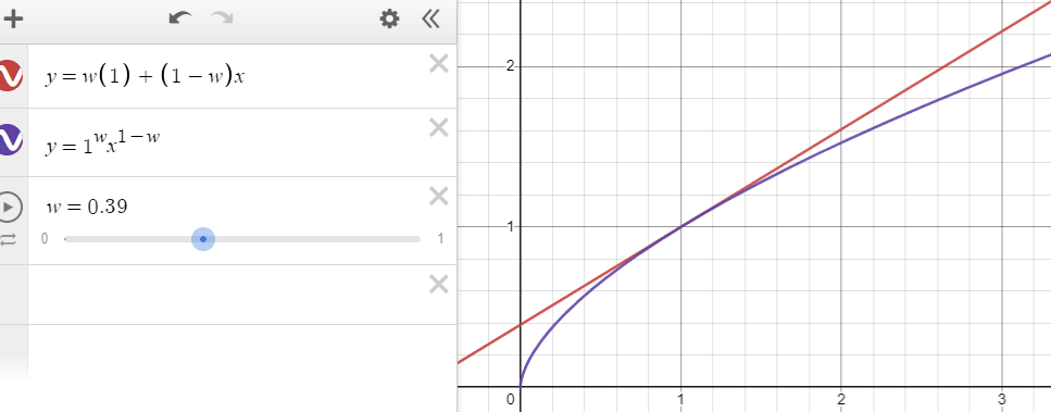
As with the unweighted means, the weighted arithmetic and geometric means are close when the ratios between estimates are low. The graph shows the two-estimate example, where the x-value is the ratio between the sub-estimates:

Again, I would argue that the geometric mean is generally superior. When the sub-estimates are close it hardly matters, and when they are far apart the geometric mean better captures the positive skew in the underlying distribution.

General findings: aggregate estimates

• When the ratio between the inputs is <3, the geometric and arithmetic means are similar. Since the arithmetic mean is more widely understood, it might be a better choice when the ratio between inputs is low.
• As the ratio between inputs grows, the means diverge. The geometric mean is superior because it captures the likely positive skew in the underlying distribution, although it may exaggerate the effect of skew.

Conclusion: complexity vs legibility

We have seen a common theme throughout: simple methods show high fidelity in situations of low variability (as measured by the ratio between confidence interval bounds or of sub-estimates).

So I would make the following suggestion: If your work is for public scrutiny or is time-sensitive, only use the more complex methods when it makes a significant difference.

• Point estimates are fine if your final calculation is not too long and the ratio between 90% confidence interval bounds is less than 2 (or if you don't need to divide by an unknown and you don't care about the "shape" of your answer).
• The normal distribution is easier to understand than lognormal, so favour it when the ratio between confidence interval bounds is low
• The arithmetic mean is widely understood, so use it as long as most of the inputs vary by less than a factor of 2

On the other hand, simple methods can lead to spurious results in situations of super-high variability. For example, estimates for the incidence of intelligent life in the galaxy (a high variability, multi-stage calculation) vary wildly depending on the complexity of the methods used.

Thanks to the makers of Squiggle, which has made working with more complex models much faster.

Changes

• [23 Mar] Amended point-estimate section to reflect that multiplication is fine with point estimates, while division introduces error. Changed summaries accordingly. Thanks to @Thomas Sepulchre [LW · GW] (LessWrong) for the comment.

5 comments

Comments sorted by top scores.