UML VI: Stochastic Gradient Descent

post by Rafael Harth (sil-ver) · 2020-01-12T21:59:25.606Z · LW · GW · 0 comments

Contents

  Gradient Descent
  Stochastic Gradient Descent
  Deriving an upper-bound on the Error
    The plan
    Step 1
    Step 2
    Step 3
    The algebraic stuff
    Reflections
None
No comments

(This is part six in a sequence on Machine Learning based on this book. Click here [LW · GW] for part 1.)

Stochastic Gradient Descent is the big Machine Learning technique. It performs well in practice, it's simple, and it sounds super cool. But what is it?

Roughly, Gradient Descent is an approach for function minimization, but it generally isn't possible to apply it to Machine Learning tasks. Stochastic Gradient Descent, which is Gradient Descent plus noise, is a variant which can be used instead.

Let's begin with regular Gradient Descent.

Gradient Descent

Given a function $f:R^d\to R$ and a point $x\in R^d$, the gradient of $f$ at $x$ is the vector of partial derivatives of $f$ at $x$, i.e.  

$\nabla f\left(x\right)=\left(\frac{\partial f}{\partial x_1}\right(x),...,\frac{\partial f}{\partial x_d}(x\left)\right)$

So the gradient at a point is an element of $R^d$. In contrast, the gradient itself (not yet applied to a point) is the function $\nabla f:R^d\to R^d$ defined by the above rule. Going forward, gradient always means "gradient at a point".

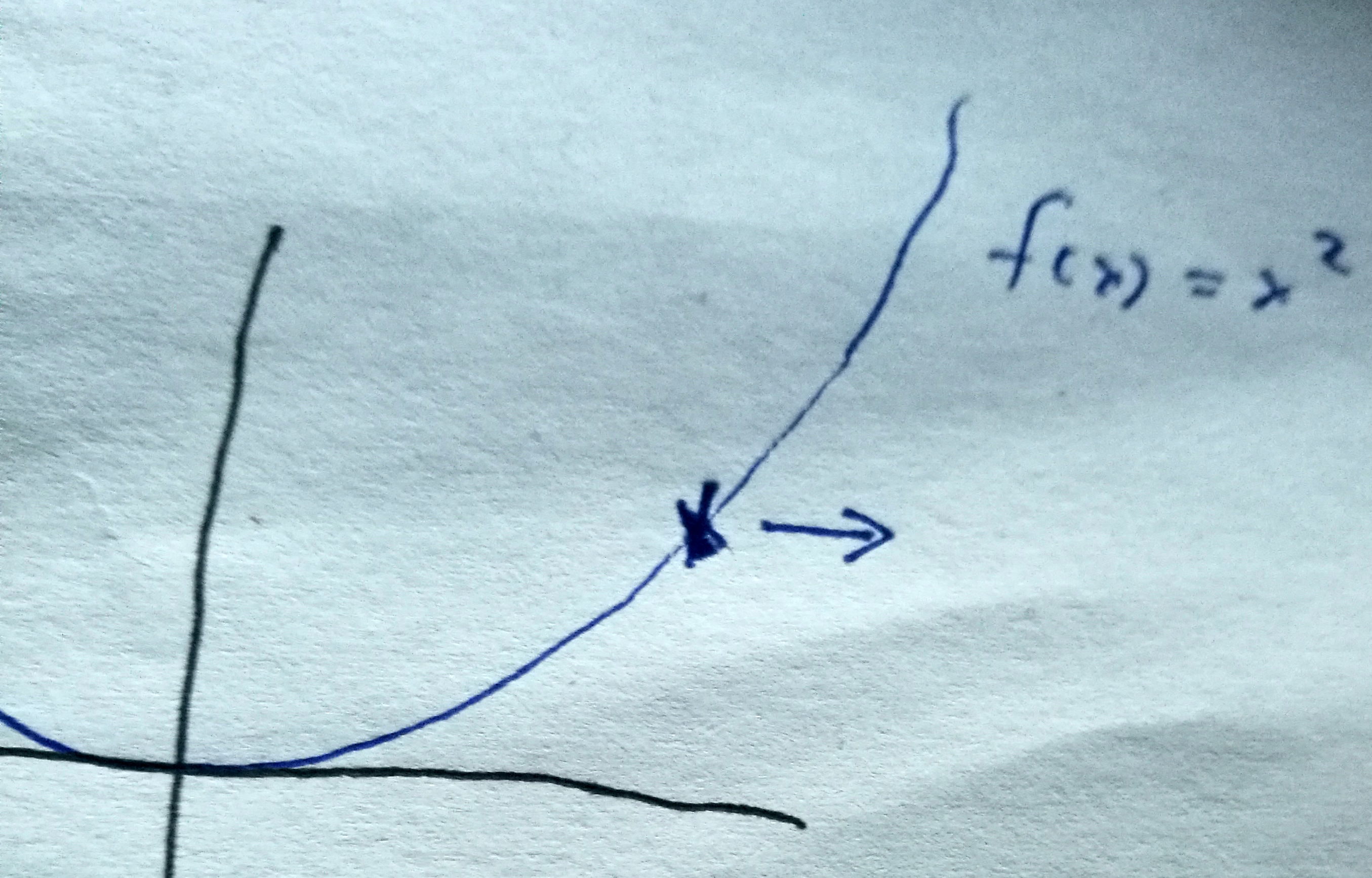
If $d=1$, then the gradient will be $f^{\prime }\left(x\right)$, a number in $R$. It can look like this:

$\to$

Or like this:

$\leftarrow$

Or also like this:

$⟶$

Point being, if $f^{\prime }\left(x\right)>0$ it'll point rightward and if $f^{\prime }\left(x\right)<0$ it'll point leftward, also it can have different lengths, but that's it. The idea of gradient descent is that the gradient points into the direction of fastest positive change, thus the opposite of the gradient is the direction of fastest negative change. It follows that, to minimize a function, one can start anywhere, compute the gradient, and then move into the opposite direction.

In the above example, the function goes up, therefore the derivative is positive, therefore the gradient points rightward. Gradient Descent tells us to go into the opposite direction, i.e. leftwards. Indeed, leftward is where the function decreases. Clearly, this is a display of utter brilliance.

Importantly, note that the picture is misleading insofar as it suggests there are more directions than two. But actually, the gradient lives in the domain space, in this case, $R$, not in the Cartesian product of domain space and target space, in this case, $R^2$. Therefore, it cannot point upward or downward.

As silly as the one-dimensional case is, it quickly becomes less trivial as we increase the dimension. Consider this function (picture taken from Wikipedia):

Again, the gradient lives in the domain space, which is $R^2$, as this image illustrates nicely. Thus it cannot point upward or downward; however, it can point into any direction within the flat plane. If we look at a point on this function, it is not immediately obvious in which direction one should move to obtain the fastest possible decrease of its function value. But if we look at the little arrows (the gradients at different domain points), they tell us the direction of the fastest positive change. If we reverse them, we get the direction of the fastest negative change.

The following is important to keep in mind: in the context of Machine Learning, the domain space for our loss function is the space of all possibe hypotheses. So the domain is itself a function space. What we want to do is to minimize a function (a loss function) that takes a function (a predictor, properly parametrized), as an argument, and outputs the performance of that predictor on the real world. For example, if we allow predictors of the form $h\left(x\right)=a{x}^2+bx+c$ for a regression problem, i.e. $X=Y=R$, our function space could be $H=R^3$, where each $(a,b,c)\in H$ defines one predictor $h_{(a,b,c)}$. Then, there is some well-defined number $\ell \left(\right(a,b,c\left)\right)$ that evaluates the performance of $h_{(a,b,c)}$ in the real world. Furthermore, if $\ell$ is differentiable, there is also some well-defined three-dimensional vector $\nabla \ell \left(\right(a,b,c\left)\right)$. The vector, which lives in $H$, tells us that the real error increases most quickly if we change the predictor in the direction of the gradient – or equivalently, that it decreases most quickly if we change the predictor in the direction opposite to the gradient. This is why we will refer to our elements of $H$ by the letters $a,b,c,a,b,c$ and such; not $x$ or $x$.

If the loss function were known, one could thus minimize it by starting with an arbitrary predictor parametrized by $a^{\left(0\right)}$, computing the gradient $\nabla \ell \left(a^{\left(0\right)}\right)$, and then "moving" into the direction opposite to the gradient, i.e. setting $a^{\left(1\right)}:=a^{\left(0\right)}-\eta \cdot \nabla \ell \left(a^{\left(0\right)}\right)$, where $\eta \in R_{+}$ is a parameter determining the step size. There is no telling how long moving into the direction opposite to the gradient will decrease the function, and therefore the choice of $\eta$ is nontrivial. One might also decrease it over time.

But, of course, the loss function isn't known, which makes regular Gradient Descent impossible to apply.

Stochastic Gradient Descent

As always, we use the training sequence $S=\left(\right(x_1,y_1),...,(x_m,y_m\left)\right)$ as a substitute for information on the real error, because that's all we have. Each element $(x,y)$ defines the point-based loss function ${\ell }_{(x,y)}:H\to R$, which we can actually use to compute a gradient. Here, $H$ has to be some familiar set – and to apply the formal results we look at later, it also has to be bounded, so think of $H=B_d(0,M)=\{x\in R^d|||x||\le M\}$.

Now we do the same thing as described above, except that we evaluate the performance of our predictor at only a single point at a time – however, we will use a different point for each step. Thus, we begin with some $a^{\left(0\right)}\in H$ which defines a predictor $h_{a^{\left(0\right)}}$, and we will update it each step so that, after step $t$, we have the predictor $h_{a^{\left(t\right)}}$. To perform step $t$, we take the loss function ${\ell }_{(x_t,y_t)}:H\to R$ which maps each $a\in H$ onto the error of the predictor $h_a$ on $(x_t,y_t)$. We compute the gradient of this loss function at our current predictor, i.e. we compute $\nabla {\ell }_{(x_t,y_t)}\left(a^{(t-1)}\right)$. Then we update $a^{(t-1)}$ by doing a small step in the direction opposite to this gradient. Our complete update rule can be expressed by the equation

$a^{\left(t\right)}:=a^{(t-1)}-\eta \cdot \nabla {\ell }_{(x_t,y_t)}\left(a^{(t-1)}\right)$

The reason why, as the book puts it, Stochastic Gradient Descent can be used to "minimize the loss function directly" is that, given the i.i.d. assumption, the point $(x_t,y_t)$ is an unbiased estimate of the real distribution, and therefore, one can prove that the expected value – with respect to the point $(x_t,y_t)$ – of the gradient we compute equals the gradient of the real loss function $\ell$. Thus, we won't always update into the right direction, but we will update into the right direction $+$ noise. The more steps one does, the lower the expected total noise will be, at least if $\eta$ is decreased over time. (This is so because, if one does random steps from some origin, then as the number of steps increases, even though the expected absolute distance from the origin will increase, the expected relative distance decreases. The expected relative distance is the term $\frac{\text{expected absolute distance}}{\text{number of steps}}$, which is an analog to $\frac{\text{expected net total noise}}{\text{number of steps}}$ in our case. Then, since we have this consistent movement into the correct direction that grows linearly with "number of steps", the term $\frac{\text{expected net total noise}}{\text{expected net total movement}}$ also decreases, making us likely to converge toward the solution.)

In the context of supervised learning, i.e. where training data is available at all, the only things that needs to hold in order for Stochastic Gradient Descent to be applicable is that (a) the hypothesis class can be represented as a familiar set, and (b) we can compute gradients on the point-based loss functions (in practice, they don't even necessarily need to be differentiable at every point). The remaining question is whether or not it will perform well. The most important property here is certainly the convexity of the loss function because that is what guarantees that the predictor will not get stuck in a local minimum, which could otherwise easily happen (the negative gradient will just keep pushing us back toward that local minimum).

In the previous chapter, we introduced the classes of convex Lipschitz bounded and convex smooth bounded problems. For both of these, one can derive upper-bounds on the expected error of a classifier trained via stochastic gradient descent for a certain number of steps. In the remainder of this chapter, we will do one of those proofs, namely the one for convex smooth bounded problems. This is an arbitrary choice; both proofs are technical and difficult, and unfortunately also quite different, so we're not doing both.

Deriving an upper-bound on the Error

The proof which upper-bounds the expected real error is of the kind that I usually don't work out in detail because it just doesn't seem worth it. On the other hand, I don't want difficult proofs to be excluded in principle. So this will be an experiment of how my style of dissecting each problem until its pieces are sufficiently small works out if applied to a proof that seems to resist intuitive understanding. In any case, working through this proof is not required to understand Stochastic Gradient Descent, so you might end this chapter here.

Now let us begin.

The plan

Recall that we wish are given a problem out of the class of convex smooth bounded [LW · GW] problems (with parameters $\beta ,M$), and we run the algorithm $A_{\text{SGD}}$ defined earlier in this post on our training sequence, $S$. We wish to bound the (expected) real error of $A_{\text{SGD}}\left(S\right)$.

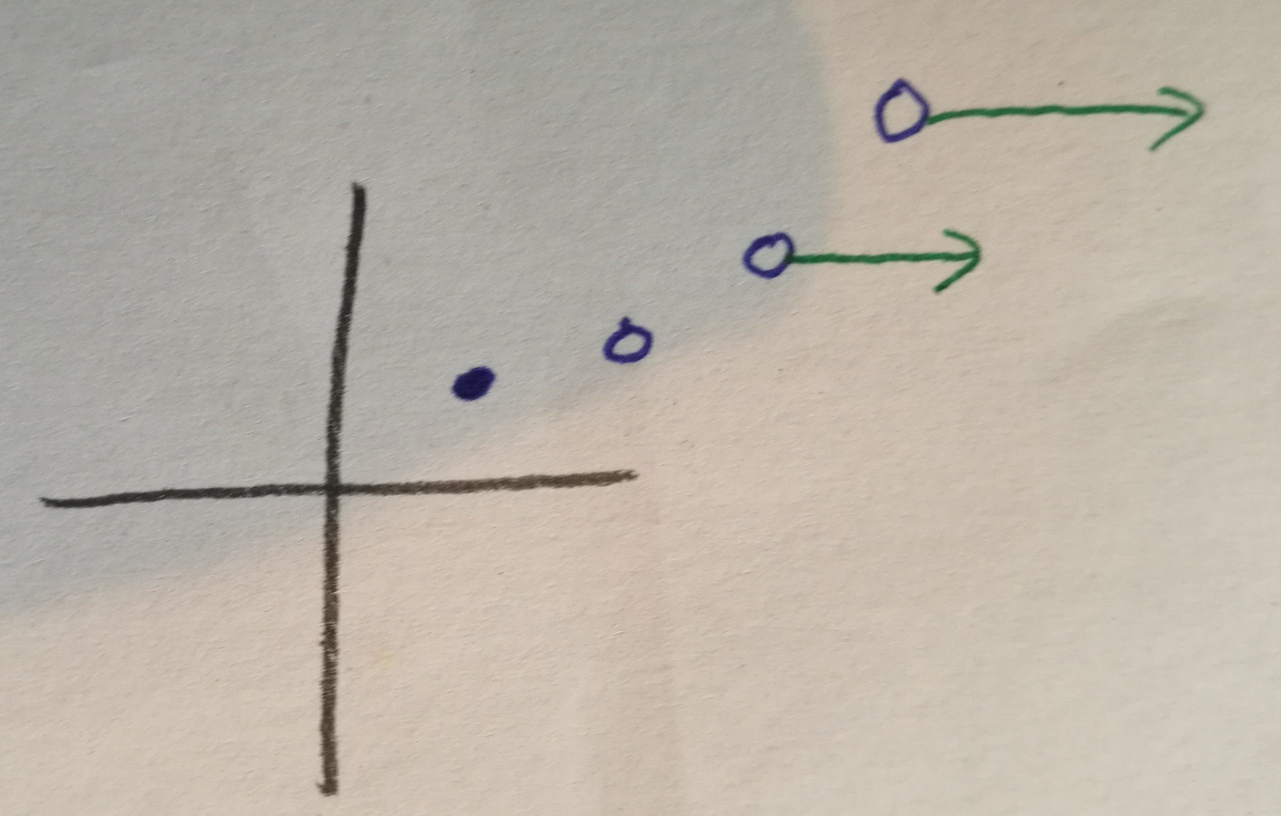
Meet the problem instance:

Of course, this is merely the problem instance within the images-world; the symbolic world where the actual proof happens will make no assumptions about the nature of the problem. That said, in the problem instance, we have $d=1$ and $m=2$, because that's enough to illustrate the steps. Our training sequence (not shown!) consists of two elements, i.e. $S=\left(\right(x_0,y_0),(x_1,y_1\left)\right)$, this time indexed from 0 to avoid having to write a lot of "$-1$". For our hypothesis class, think of $H=[-10,10]$, where each $a\in H$ defines a simple linear predictor $h_a$ – although going forward, we will pretend as if $a$ itself is the predictor. What the picture does show is the predictors $a^{\left(0\right)}\to a^{\left(1\right)}\to a^{\left(2\right)}$ through which the algorithm iterates (the highest one is $a^{\left(0\right)}$, the second-highest $a^{\left(1\right)}$, and the one without a gradient arrow is $a^{\left(2\right)}$). They live in $1$-dimensional space (on the $x$-axis). Their real error corresponds to their position on the $y$-axis. Thus, both the predictors themselves and their errors are monotonically decreasing. The green arrows denote the gradients $\nabla {\ell }_{(x_0,y_0)}\left(a^{\left(0\right)}\right)$ and $\nabla {\ell }_{(x_1,y_1)}\left(a^{\left(1\right)}\right)$. The filled point denotes the optimal predictor $a^{\ast }$.

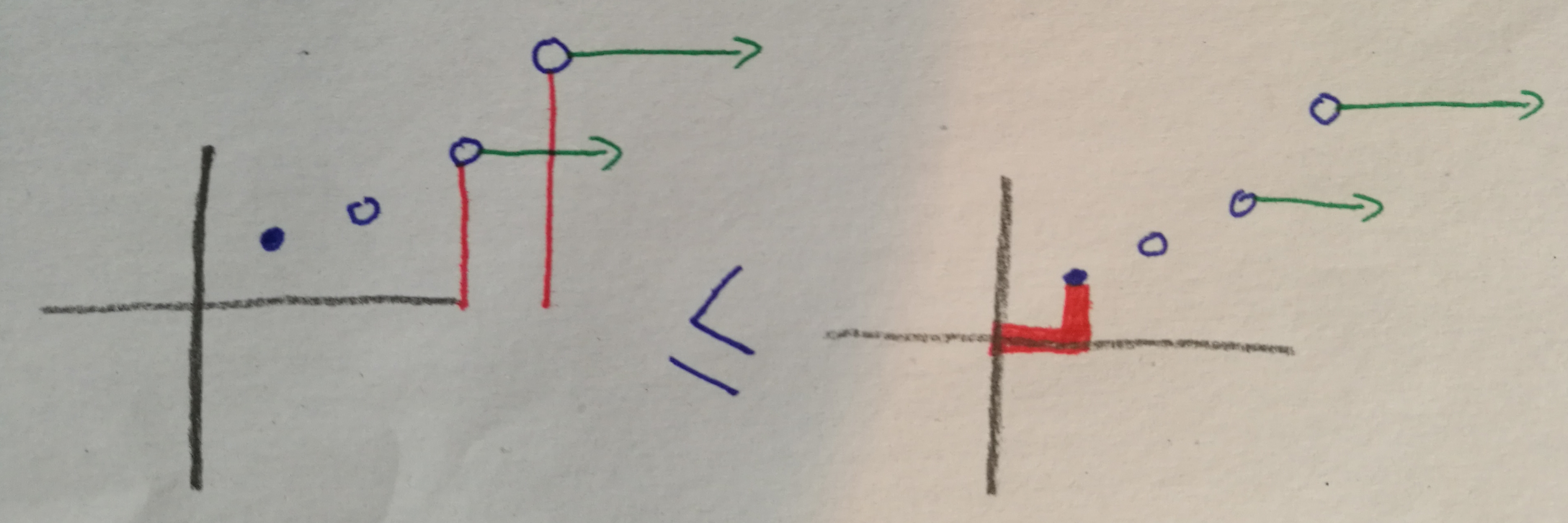
For unspecified reasons – probably because it makes analysis easier, although it could also reduce variance in practice – the precise algorithm we analyze puts out the predictor $\frac{1}{m}{\sum }_{i=0}^{m-1}{a}^{\left(i\right)}$ rather than $a^{\left(m\right)}$, even though $a^{\left(m\right)}$ naively looks like the better choice. In our case, that means we put out $\frac{1}{2}(a^{\left(0\right)}+a^{\left(1\right)})$. With that in mind, now meet the proof roadmap:

The proof roadmap illustrates what terms we're concerned with (red), and which upper-bounds we're deriving. Dashed lines mean a small $(<1)$ factor in front of the term; fat lines mean a large $(>1)$ factor. In the beginning, we look at the difference between the error of our output predictor $\frac{1}{2}(a^{\left(0\right)}+a^{\left(1\right)})$ and that of the optimal predictor $a^{\ast }$ (leftmost picture). Then we do three steps; in each step, we bound our current term by a different term. First, we bound it in terms of the inner product between the predictors themselves and the gradients. Then, we bound that by $\delta$ times the norm of the gradients plus many times the norm of the optimal predictor, where $\delta <1$. Then we bound that by $\delta$ times the total error of our output predictor plus a lot of times the norm of the optimal predictor.

At that point, we've made a circle. Well – not quite, since we started with the difference between the error of the output predictor and that of the optimal predictor (hence why the lines don't go all the way down in picture one) and ended with the total error of the output predictor. But it's good enough. Through algebraic manipulations (adding the error of the optimal predictor on both sides and rescaling), we obtain a bound on the error of our output predictor, in terms of the error of the optimal predictor and the norm of the optimal predictor, i.e.:

And the equation corresponding to this picture will be the theorem statement.

Now we just have to do the three steps, and then the algebraic stuff at the end.

Step 1

We start by bounding the term ${\sum }_{t=0}^{T-1}\left[{\ell }_{(x_t,y_t)}\right(a^{\left(t\right)})-\ell (a^{\ast }\left)\right]$, which is closely related to but not identical to the real error of the output predictor (it is defined in terms of the point-based loss functions rather than the real error). $T$ will be the number of steps, so $T=m$. Recall the proof roadmap:

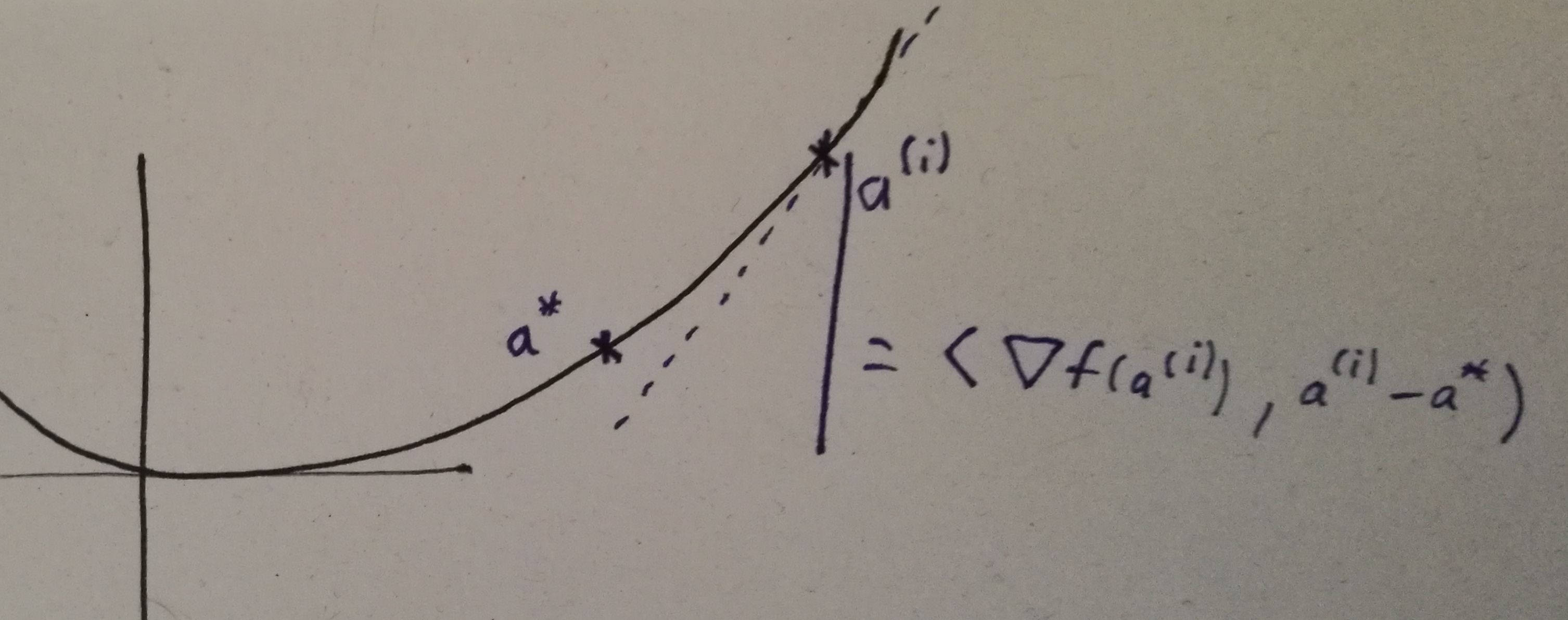
The first stop (second picture) is the term ${\sum }_{t=0}^{T-1}⟨a^{\left(t\right)}-a^{\ast },{\nabla }_t⟩$, where we write ${\nabla }_t$ for $\nabla {\ell }_{(x_t,y_t)}\left(a^{\left(t\right)}\right)$. This bound applies for each summand individually, and it relies on a fundamental property of convex functions, namely that every tangent remains below the function:

This should be easy enough to believe; let's skip the formal proof and continue.

Step 2

Our current term is ${\sum }_{t=0}^{T-1}⟨a^{\left(t\right)}-a^{\ast },{\nabla }_t⟩$. Recall the proof roadmap:

The next stop (third picture) is the term $\frac{1}{2\eta }||a^{\ast }|{|}^2+\frac{\eta }{2}{\sum }_{t=0}^{T-1}||{\nabla }_t|{|}^2$. This will be the hardest step – let's begin by reflecting on what it means.

We wish to bound the inner product of predictors and corresponding gradients with the norm of the gradients and the norm of the final predictor. So what we lose is the values of the predictors themselves. However, these are implicit in the gradients, since they encode how we move toward our final predictor (or equivalently, how we move away from the final predictor). Consequently, we will need to use the update rule, $a^{(t+1)}=a^{\left(t\right)}-\eta {\nabla }_t$, to prove this result.

Our approach will be to reduce the inner product $⟨a^{\left(t\right)}-a^{\ast },{\nabla }_t⟩$ to the difference between $||a^{\left(t\right)}-a^{\ast }|{|}^2$ and $||a^{(t+1)}-a^{\ast }|{|}^2=||a^{\left(t\right)}-\eta {\nabla }_t-a^{\ast }|{|}^2$. Alas,

$||a^{\left(t\right)}-a^{\ast }|{|}^2-||a^{\left(t\right)}-\eta {\nabla }_t-a^{\ast }|{|}^2=2⟨a^{\left(t\right)},\eta {\nabla }_t⟩-2⟨a^{\ast },\eta {\nabla }_t⟩-⟨\eta {\nabla }_t,\eta {\nabla }_t⟩$

Or differently written, $⟨a^{\left(t\right)}-a^{\ast },2\eta {\nabla }_t⟩-{\eta }^2||{\nabla }_t|{|}^2$. Thus, we have

$⟨a^{\left(t\right)}-a^{\ast },{\nabla }_t⟩=\frac{1}{2\eta }⟨a^{\left(t\right)}-a^{\ast },2\eta {\nabla }_t⟩=\frac{1}{2\eta }(||a^{\left(t\right)}-a^{\ast }|{|}^2-||a^{(t+1)}-a^{\ast }|{|}^2+{\eta }^2||{\nabla }_t|{|}^2)$

Then, ${\sum }_{t=0}^{T-1}⟨a^{\left(t\right)}-a^{\ast },{\nabla }_t⟩=\frac{1}{2\eta }{\sum }_{t=1}^{T-1}||a^{\left(t\right)}-a^{\ast }|{|}^2-||a^{(t+1)}-a^{\ast }|{|}^2+{\eta }^2||{\nabla }_t|{|}^2$, and the first two elements of this are a telescopic sum, i.e. each segment negates part of the next segment. What remains is $\frac{1}{2\eta }(||a^{\left(0\right)}-a^{\ast }|{|}^2-||a^{\left(T\right)}-a^{\ast }|{|}^2+{\sum }_{t=0}^{T-1}{\eta }^2||{\nabla }_t|{|}^2)$, and we can upper bound it as $\frac{1}{2\eta }||a^{\ast }|{|}^2+{\sum }_{t=0}^{T-1}\frac{\eta }{2}||{\nabla }_t|{|}^2$, which is the bound we wanted to have. Here, the $a^{\left(0\right)}$ disappeared because the algorithm assumes we start with $a^{\left(0\right)}=0$, which I conveniently ignored in my drawings.

Step 3

Our current term is $\frac{1}{2\eta }||a^{\ast }|{|}^2+\frac{\eta }{2}{\sum }_{t=0}^{T-1}||{\nabla }_t|{|}^2$. Recall the proof roadmap:

The next stop (last picture) is the term $\frac{1}{2\eta }||a^{\ast }|{|}^2+\beta \cdot \eta {\sum }_{t=0}^{T-1}{\ell }_{(x_t,y_t)}\left(a^{\left(t\right)}\right)$. This one will also work for each summand separately. We wish to prove that

$||{\nabla }_t|{|}^2=||\nabla {\ell }_{(x_t,y_t)}\left(a^{\left(t\right)}\right)|{|}^2\le 2\beta \cdot {\ell }_{(x_t,y_t)}\left(a^{\left(t\right)}\right)$,

where $\beta$ is from the smoothness definition of our point-wise loss function. So this bound is all about smooth functions. It even has a name: functions with this property are called self-bounded, because one can bound the value of the gradient in terms of the value of the same function.

If one were to prove this formally, one would do so for arbitrary smooth functions, so one would prove that, if $O\subseteq R^d$, where $O$ is convex, and $f:O\to R$ is a $\beta$-smooth and nonnegative function, then

$||\nabla f\left(x\right)|{|}^2\le 2\beta \cdot f\left(x\right)\forall x\in O$

Recall that $f$ is $\beta$-smooth iff $||\nabla f\left(x\right)-\nabla f\left(y\right)||\le \beta ||x-y||$ for all $x$ and $y$. Now, why is this statement true? Well, if we imagine $f$ to model the position of a space ship, then smoothness says that $f$ cannot accelerate too quickly, so in order to reach a certain speed, it will gradually have to accelerate towards that point and thus will have to bridge a certain distance. Let's take the one-dimensional case, and suppose we start from $0$ and consistently accelerate as fast as we're allowed to (this should be the optimal way to increase speed while minimizing distance). Then $f\left(x\right)=0$ and $f^{\prime \prime }\left(x\right)=\beta$, which means that $f^{\prime }\left(x\right)=\beta x$ and $f\left(x\right)=\frac{1}{2}\beta x^2$; then $f^{\prime }(x{)}^2=(\beta x{)}^2=2\beta \cdot \frac{1}{2}\beta x^2=2\beta f\left(x\right)$. This is reassuring, because we've tried to construct the most difficult case possible, and the statement held with equality.

The formal proof, at least the one I came up with, is quite long and relies on line integrals, so we will also skip it.

The algebraic stuff

We have established that

${\sum }_{t=0}^{T-1}\left[{\ell }_{(x_t,y_t)}\right(a^{\left(t\right)})-\ell (a^{\ast }\left)\right]\le \frac{1}{2\eta }||a^{\ast }|{|}^2+\beta \cdot \eta {\sum }_{t=0}^{T-1}{\ell }_{(x_t,y_t)}\left(a^{\left(t\right)}\right)$

which can be reordered as

${\sum }_{t=0}^{T-1}{\ell }_{(x_t,y_t)}\left(a^{\left(t\right)}\right)\le \frac{1}{2\eta }||a^{\ast }|{|}^2+\beta \cdot \eta {\sum }_{t=0}^{T-1}{\ell }_{(x_t,y_t)}\left(a^{\left(t\right)}\right)+{\sum }_{t=0}^{T-1}\ell \left(a^{\ast }\right)$.

At this point, we better have that $\beta \eta <1$, otherwise, this bound is utterly useless. Assuming $\eta \beta <1$ does indeed hold, we can further reformulate this equation as

$(1-\beta \eta ){\sum }_{t=0}^{T-1}{\ell }_{(x_t,y_t)}\left(a^{\left(t\right)}\right)\le \frac{1}{2\eta }||a^{\ast }|{|}^2+T\cdot \ell \left(a^{\ast }\right)$

Rescaling this, we obtain

${\sum }_{t=0}^{T-1}{\ell }_{(x_t,y_t)}\left(a^{\left(t\right)}\right)\le \frac{1}{(1-\beta \eta )}(T\cdot \ell \left(a^{\ast }\right)+\frac{1}{2\eta }||a^{\ast }|{|}^2)$

Dividing this by $T$ to have the left term closer to our actual error, we get

$\frac{1}{T}{\sum }_{t=0}^{T-1}{\ell }_{(x_t,y_t)}\left(a^{\left(t\right)}\right)\le \frac{1}{(1-\beta \eta )}(\ell \left(a^{\ast }\right)+\frac{1}{2\eta T}||a^{\ast }|{|}^2)$.

Now we take expectations across the randomization of the training sequence $S$ on both sides. Then the left side becomes the expected real error of our output predictor $A_{\text{SGD}}\left(S\right)=\frac{1}{m}{\sum }_{i=0}^{m-1}{a}^{\left(i\right)}$. The right term doesn't change, because it doesn't depend on $S$. Thus, we have derived the bound

$E\left(A_{\text{SGD}}\right(S\left)\right)\le \frac{1}{(1-\beta \eta )}(\ell \left(a^{\ast }\right)+\frac{1}{2\eta T}||a^{\ast }|{|}^2)$

and this will be our final result. By choosing $\eta$ correctly and rearranging, it is possible to define a function $s^{\ast }$ such that, for any $\beta$ and $M$ upper-bounding the hypothesis class ($||a^{\ast }||$ cannot be an input since we don't know the optimal predictor $a^{\ast }$) and any arbitrarily small $ϵ\in R_{+}$, if $T\ge s^{\ast }(\beta ,M,ϵ)$, then the above is upper-bounded by $\ell \left(a^{\ast }\right)+ϵ$. To be specific, $s^{\ast }$ will be given by $s^{\ast }(\beta ,M,ϵ)=12\cdot M^2\cdot \beta \cdot \frac{1}{{ϵ}^2}$.

Reflections

Recall that $\beta$ is the parameter from the smoothness of our loss function, $T$ is the number of training steps we make (which equals the number of elements in our training sequence), and $\eta$ is the step size, which we can choose freely. In the result, we see that a smaller $\beta$ is strictly better, a larger $T$ is strictly better, and $\eta$ will have its optimum at some unknown point. This all makes perfect sense – if things had come out any other way, that would be highly surprising. Probably the most non-obvious qualitative property of this result is that the norm of the optimal predictor plays the role that it does.

The most interesting aspect of the proof is probably the "going around in a circle" part. However, even after working this out in detail, I still don't have a good sense of why we chose these particular steps. If anyone has some insight here, let me know.

0 comments

Comments sorted by top scores.