Extracting SAE task features for in-context learning
post by Dmitrii Kharlapenko (dmitrii-kharlapenko), neverix, Neel Nanda (neel-nanda-1), Arthur Conmy (arthur-conmy) · 2024-08-12T20:34:13.747Z · LW · GW · 1 commentsContents
  TL;DR
  Prior work
  Initial Phi-3 experiments
    Direct SAE task vector reconstruction
    Task-related SAE features
    Task vector SAE cleanup
    Early layer task vector cleanup
  Further experiments on Gemma 1 2B
    Comparison with task vectors
    Task features
    Task detector features
  Next steps
  How gradient-based task vector cleanup can be used
  Acknowledgements
None
1 comment
TL;DR
- We try to study task vectors in the SAE basis. This is challenging because there is no canonical way to convert an arbitrary vector in the residual stream to a linear combination of SAE features — you can't just pass an arbitrary vector through the encoder without going off distribution.
- We explored the algorithm of gradient pursuit suggested in Smith et al [AF · GW], but it didn’t work for us without modifications.
- Our approach is to apply the SAE encoder to the task vector, and then apply a gradient-based cleanup. This exploits the fact that task vectors have a differentiable objective. We find that this gives a sparser and cleaner reconstruction, which is also highly interpretable, and also serves as a better task vector due to directly optimizing for log likelihood. This takes us from ~100 active features to ~10.
- Using our algorithm, we find two classes of SAE features involved in ICL. One of them recognizes the exact tasks or output formats from the examples, and another one encodes the tasks for execution by the model later on. We show that steering with these features has causal effects similar to task vectors.
This work was produced as part of the ML Alignment & Theory Scholars Program - Summer 24 Cohort, under mentorship from Neel Nanda and Arthur Conmy.
Prior work
Task or function vectors are internal representations of some task that LLMs form while processing an ICL prompt. They can be extracted from a model running on a few-shot prompt and then be used to make it complete the same task without having any prior context or task description.
Several papers (Function vectors in large language models, In-Context Learning Creates Task Vectors) have proposed different ways to extract those task vectors. They all center around having ICL examples being fed to a model in the form of “input <separator> output, … ” and averaging the residuals on the “separator” token over a batch. This approach can reconstruct some part of the ICL performance but does not admit a straightforward conversion to the SAE basis.
ITO with gradient pursuit [? · GW] can be used to do a sparse coding of a residual vector using SAE features. The post suggests using this algorithm for steering vector SAE decomposition. Since task vectors can be thought of as steering vectors, ITO may provide some insight into the ways they operate.
Initial Phi-3 experiments
Direct SAE task vector reconstruction
In our study we trained a set of gated SAEs for Phi-3 Mini 3.8B using a model-generated synthetic instruction dataset.
While offering a sparse dictionary decomposition of residuals, SAEs tend to introduce a reconstruction error that impacts the performance of the model. They also have no guarantee to be able to decompose out-of-distribution vectors, and task vectors being a product of averaging activations across prompts and tokens may be the case of such vectors.
Thus, we first studied the performance of SAE reconstructions of task vectors in transferring the definition of two tasks: 1) antonym generation and 2) English to Spanish word translation. These and other tasks used to study task vectors were taken from the ICL task vectors paper github repository.
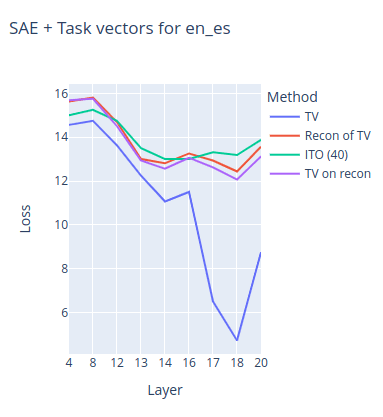
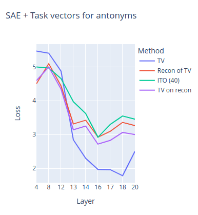
These charts show the NLL loss of the model on the evaluation set of zero-shot prompts for both of the tasks depending on the layer of extraction/insertion.
- TV stands for the original task vector performance;
- Recon of TV stands for using the SAE reconstruction of the task vector instead of the task vector;
- TV on recon stands for first doing a SAE reconstruction of the residuals and then collecting a task vector on them;
- ITO stands for the ITO algorithm with 40 target l0 loss.
It can be seen from charts that SAE reconstruction significantly decreases the performance of the task vectors. We speculate that English to Spanish is a more complex task for the model because task vectors do not work until layer ~17 compared to ~13 in the case of antonyms and thus is only represented at a more abstract level in the model. Indeed, the chart shows that SAE reconstruction almost completely destroys the task vector performance for this task.
Similar results can be seen in all of the other tasks that we tried.
Task-related SAE features
After seeing that the SAE reconstructions of task vectors do keep some of the performance, we assumed that SAE features are capable of capturing the internal task representations to some extent. And this does seem to be the case!
Here are the some of the max-activating examples for some of the SAE features in the antonyms task vector:
- 21441: federal government and individual states was
- 21885: I run around the city, but I never move.
- 22813: The company collected data on the ages and years of experience of 50 successful employees and 50 unsuccessful
- 47882: let likes = []; let hates
We also found that using just a single one of those task related features as a steering direction recovers some of the performance of the original task vector and almost matches the performance of the reconstruction. We also found that deeper layers (~18) tend to have more interpretable task-related features, even if task vectors start reliably working much earlier (layers 12-14).
Unfortunately, these task-related features were mostly buried among dense or “repeated pattern”-related features in the reconstructions. The top (and therefore first picked by gradient pursuit) ~30 features were dense in some examples.
Task vector SAE cleanup
This motivates the creation of a method that can reinforce the features from the reconstruction that have a significant impact on task performance and remove those that do not. We introduce a method called sparse SAE task vector finetuning. A diagram of the method can be seen below.
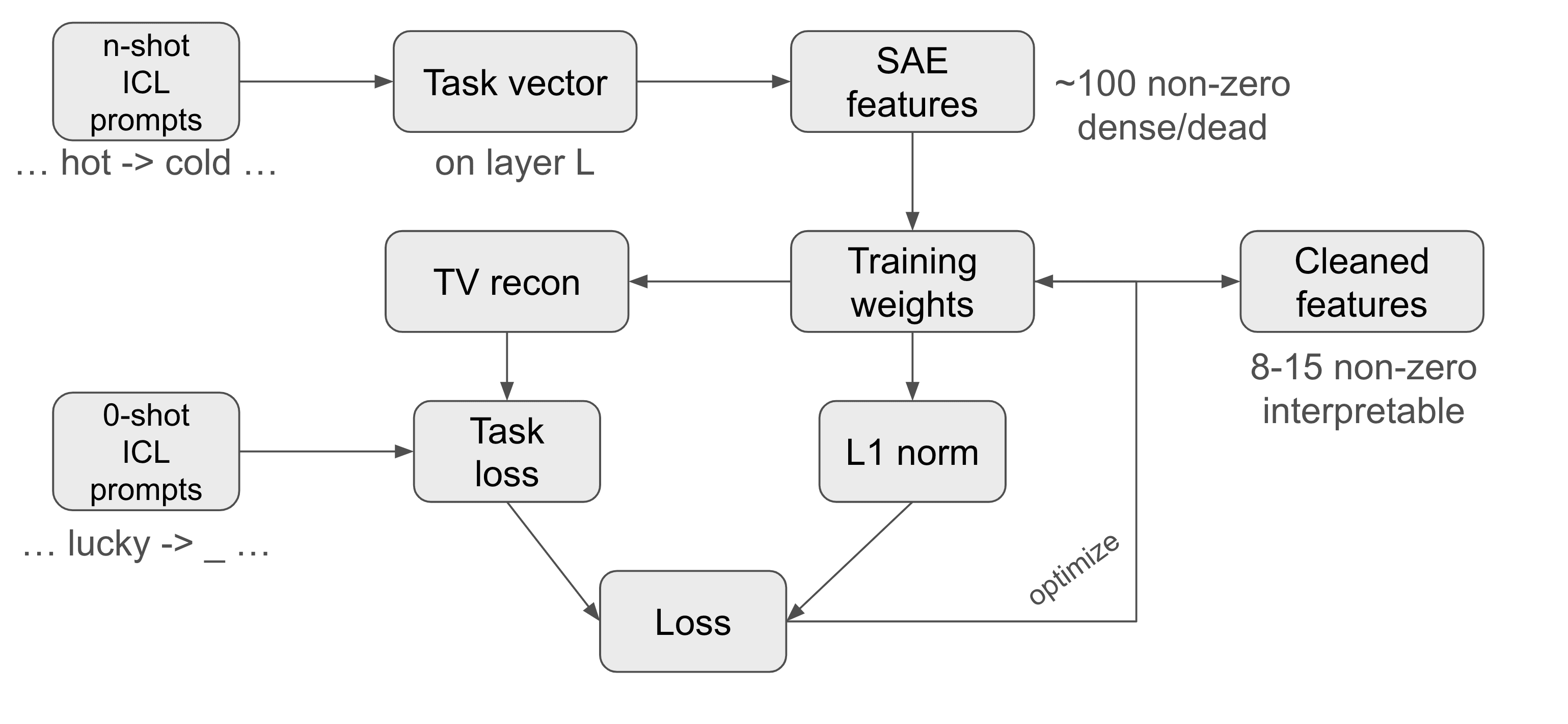
At its core, this method takes a set of zero-shot prompts and fine-tunes a residual activation addition vector at some layer with the objective of reducing the NLL loss on these prompts. However, instead of optimizing the vector directly, the method optimizes the weights of its SAE reconstruction regularized by a L1 norm of these weights. The key point is that we initialize these weights not with random values (this did not work) but with the SAE reconstruction of the task vector at the corresponding layer. And this works surprisingly well!
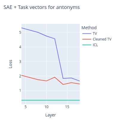
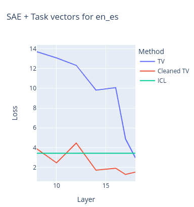
These charts contain the NLL loss on the same two tasks as the previous figure with task vectors vs cleaned task vectors depending on different extraction/insertion layers. The loss of the model on a multishot ICL prompt (used to create the task vector) is also provided as reference, although it was calculated on another set of prompts.
- TV stands for task vector loss
- Cleaned TV stands for the cleaned task vector loss
We can see that task vector cleaning not only preserves the original task vector performance, but even surpasses it. Another interesting result is that this cleanup method (surprisingly) allows task vectors to work on much earlier layers. It also drops the amount of SAE features to study from ~100 non-zero ones in the SAE reconstruction to just ~8-15. And a large portion of these features are actually task-related (as judged by us).
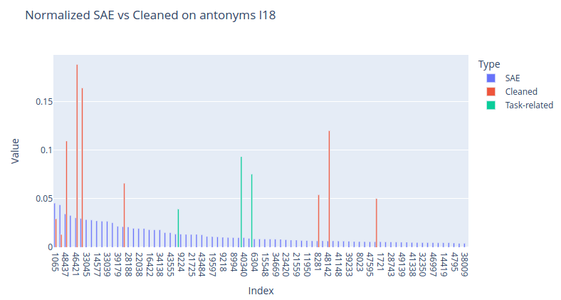
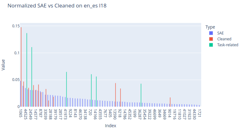
These charts show normalized features of the SAE task vector reconstructions (blue) vs cleaned task vector features (red + green). Although this method still keeps some of the dense features (and their removal significantly impacts the performance), it greatly boosts the task-related features and removes a significant portion of the useless features. These are some other task-related layer 18 features found using this method:
- en_fr
- 5794: le cuivre et le vanadium, en fonction de la qualité et des propriétés mécaniques souh aitées pour
- es_en
- 44330: To compute the norm (also known as the magnitude)
- 19597: (from the Latin, ante meridiem, meaning before midday) and p.m. (post meridiem, meaning
- country_capital
- 23218: flight from Vancouver to London earlier this
- 41579: Describe the location in which the story takes place . Par
- person_profession
- 7702: Laura Johnson: A science journalist
- location_language
- 34365: This text is in Romanian.
- 47500: The sentence "Tehkää näin, ja teette Euroopalle palveluksen" is in Finnish,
- location_religion
- 45373: is an independent Christian organization based on the Philippines and
Cleaned task vectors also seem to offer better generalization than original task vectors. For example, for a sentence-to-sentence English to Spanish translation task, the single-word English to Spanish translation task vector gives 18.125 NLL loss, but we get 14.68 with a version of the same task vector cleaned with our method (sentence pairs were taken from the Helsinki Opus dataset).
Early layer task vector cleanup
Although the cleaned task vectors are more capable of transferring the context on much earlier layers than the original task vectors, the features on these layers tend to be much less interpretable. We tried studying this a bit more in-depth by first cleaning up a Layer 4 task vector, then inserting it at the lower layer, and then looking at the residuals at Layer 18:

We found that it results in L18 task vectors that share a lot of common features with basic L18 task vectors, while having increased relative weights of task-related features[1]. This suggests that the method may actually be exploiting the internal model task vector formulation mechanism and not just finding some fine-tuning that works.
Further experiments on Gemma 1 2B
Comparison with task vectors
For our Gemma 2B experiments we also trained a full SAE suite using the FineWeb dataset.
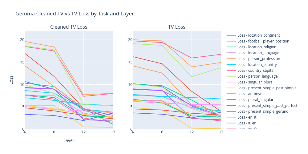
We can see that cleaned task vectros in Gemma 2B have either the same or higher performance as task vectors (regular SAE reconstruction either decreases the performance or just loses it completely).
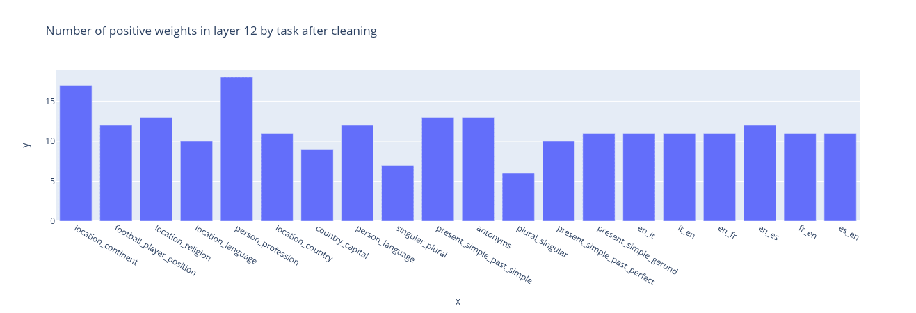
Cleaning leaves 5-15 non-zero features on layer 12 for most of the tasks.
Task features
We again notice that cleaned task vectors always contain interpretable task-related features. Often these features directly define the task, i.e. features from antonyms task vectors activate right before the model predicts the second antonym, or features from Spanish to English translation activate right before the model starts translating to English. Below are examples of some of those features.


We believe these features encode the action that the model should perform next. Task features from tasks like present_simple_past_simple reinforce this hypothesis. Their max activations come not from present simple -> past simple pairs, but just from tokens after which it is expected to have a verb in past tense. This is why we believe they are closer to “predict past simple next” features than just present simple to past simple task features. This may be also caused by the fact that the dataset for max activating examples collection did not contain such pairs.
Going further, just steering with these task features alone also recovers some of the task vector performance, and only for related tasks. For that, we use a zero-shot prompt with no explanation, and just add the scaled feature direction to the “->” (separator) token.
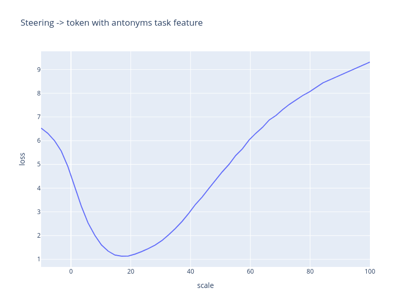
Using a scale of 20 we can see how steering with different task features affects different tasks. The chart below shows a relative loss change (with no steering taken as a base) for pairs of different tasks and task features.
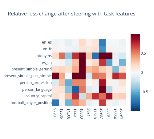
Maximum increase clipped to 1 (from 3.5)
It is possible to notice that most of the tasks here have just a single feature with high relative loss decrease. Other features either do not affect the loss at all or even increase it by several times. The exceptions are translation from English tasks, since the feature selected for them is an “English to foreign language translation” feature. In cleaned task vectors it was accompanied by features that activate on any foreign texts. We believe they are used to encode the target language.
Another notable example is the feature 13458 that improves loss on “person to some property” tasks. This may mean that it has a broader use than just recalling someone’s profession in the model.
Task detector features
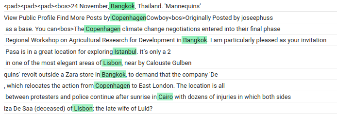
Using an algorithm similar to Sparse Feature Circuits (to be published in a future blog post), we found a second type of task-related features. These features seem to play an important role in the formation of task features. We call them task detector features. We hypothesize that they do exactly what their name implies: detect completed tasks in ICL prompts or just generic texts.


Furthermore, we can often use the task vector cleaning algorithm to find these features. For that, we first collect the task vector from the output tokens. Then we modify the zero-shot prompt to a one-shot prompt with a generic example “X -> Y” (literally). Finally, we optimize the loss after steering on the token “Y” at the layer of collection. From our experience, task vectors collected in this fashion do not usually work, while the cleaned ones often do.
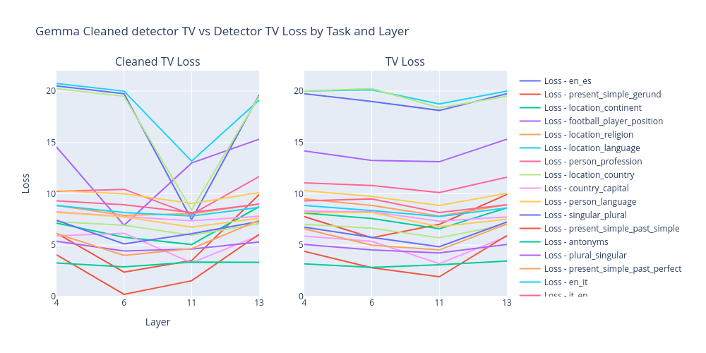
Cleaned task detector vectors seem to have a bigger impact on earlier layers than cleaned task vectors. That is expected, since task detector features can be used to construct later task features. We also note that not all features that we classify as detectors are exact task detectors. For example, a detector feature that is used in the “country to capital” task activates on capitals of different countries without any mention of the said countries. This also suggests that task features often encode tasks in a broader sense, i.e. “predict the most appropriate capital in this context”, and not just “predict the capital of this country”.
We can also plot relative loss change for pairs of different detectors and tasks. This time we will use a scale of 25.
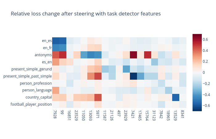
We can again see that these features have a noticeable causal effect on the task completion.
Next steps
Our current results suggest three directions for further investigation:
- How do task detectors form?
- How are they converted into task features?
- How do task features manipulate downstream execution?
We expect directions 1 and 3 to have a lot of task-specific mechanisms, and thus results from them may not generalize to a broad range of tasks. Meanwhile, direction 2 seems to be focused on interactions between feature types common to most tasks. Therefore, we are currently working on it by looking at task features with sparse feature circuits.
We may also try training our SAE features on datasets that include many more variations of ICL tasks that can distinguish features relevant for only specific tasks.
How gradient-based task vector cleanup can be used
Task vector cleanup is most promising as a way of discovering task-related SAE features, and it can specifically help find causally relevant ones without circuit discovery. It can also be seen as a fine-tuning method, and it shares some of the flaws: ease of implementation (moderate, with hyperparameter tuning needed for learning rate and sparsity coefficient) and faithfulness to the original behavior or task vector (low). It is, however, regularized: the vector is restricted to a 10-100-dimensional subspace defined by the SAE features and is encouraged to be sparse.
The method described is also somewhat similar to 1-dimensional distributed alignment search. There is a potential interpretability illusion here similar to An Interpretability Illusion for Subspace Activation Patching. Our primary method of evaluating sparse task vector fine-tuning is looking at the loss (steering metric) and presence of interpretable features (max-activating tokens being a loose estimate of correlation with a target concept). One experiment to test for this would be hand-picking interpretable features, tuning weights only and evaluating the resulting vector’s loss.
Acknowledgements
This work was produced during the research sprint of Neel Nanda’s MATS training program. We thank Neel Nanda as our mentor and Arthur Conmy as our TA. We thank McKenna Fitzgerald for research management and feedback. We are grateful to Google for providing us with computing resources through the TPU Research Cloud.
- ^
Top SAE features of L18 TV before: 1065, 33278, 48437, 24363, 46421, 8787, 33045, 26164, 14577, 46849, 33039, 46370, 39179, 47882, 28188, 33953, 22038, 28517, 16422, 11831, 34138, 16805, 43555, 21885, 9224
Top SAE features of L18 TV after: 1065, 33039, 11831, 46849, 24363, 34138, 22038, 48437, 33953, 6188, 8023, 48299, 4483, 21885, 5405, 18196, 14577, 46370, 25746, 31738, 39233, 28517, 41370, 8787, 43555
1 comments
Comments sorted by top scores.
comment by Clément Dumas (butanium) · 2024-08-13T09:58:12.265Z · LW(p) · GW(p)
Nice work!
I'm curious about the cleanliness of a task vector after removing the mean of some corrupted prompts (i.e., same format but with random pairs). Do you plan to run this stronger baseline, or is there a notebook/codebase I could easily tweak to explore this?
