Topological Data Analysis and Mechanistic Interpretability
post by Gunnar Carlsson (gunnar-carlsson) · 2025-02-24T19:56:02.498Z · LW · GW · 4 commentsContents
  I. Topological Data Modeling
  II. Mapper
  III. Mechanistic Interpretability
  IV. Graph Modeling of SAE features
  V. Next steps for TDA and SAE features
  VI. Summary
  VII. Acknowledgments
None
4 comments
This article was written in response to a post on LessWrong from the Apollo Research interpretability team [LW · GW]. This post represents our initial attempts at acting on the topological data analysis suggestions.
In this post, we’ll look at some ways to use topological data analysis (TDA) for mechanistic interpretability. We’ll first show how one can apply TDA in a very simple way to the internals of convolutional neural networks to obtain information about the “responsibilities” of the various layers, as well as about the training process. For LLM’s, though, simply approaching weights or activations “raw” yields limited insights, and one needs additional methods like sparse autoencoders (SAEs) to obtain useful information about the internals. We will discuss this methodology, and give a few initial examples where TDA helps reveal structure in SAE feature geometry.
I. Topological Data Modeling
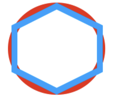
The term topology refers to the study of shape using methods that are insensitive to deformations such as stretching, compressing, or shearing. For example, topology does not “see” the difference between a circle and an ellipse, but it does recognize the difference between the digit 0 and the digit 8. No matter how I stretch or compress the digit 0, I can never achieve the two loops that are present in the digit 8. Shapes can often be represented by graphs or their higher dimensional analogues called simplicial complexes. For instance, one can think of a hexagon as modeling a circle, with the understanding that the modeling is accomplished with a small amount of error:
Of course data sets can have notions of shape, too. For example, here is a data set that we can recognize as having a circular shape, even though it only consists of samples and is not a complete circle.
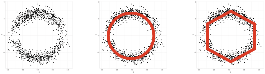
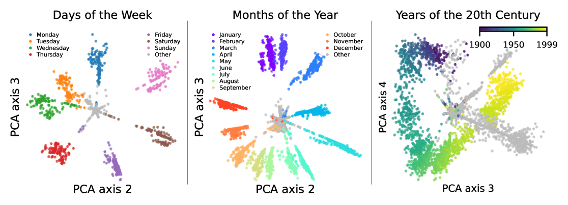
A circular shape may be an indication of periodic behavior. In a mechanistic interpretability context, Engels et al showed that some LLM SAE features are organized in a circular pattern, and that those features correspond to temporal periodic structures like days of the week or months of the year.
There are numerous other examples where periodic data is shown as a circle when graphed, notably in dynamical systems like predator/prey models.
II. Mapper
Mapper is the name for a family of methods that use topological ideas to build graphs representing data sets. The core concept behind Mapper is the nerve of a covering. A covering of a set is a family of subsets so that . The nerve graph of the covering is the graph whose vertices correspond to the sets , and where vertices and form an edge in if , i.e. if and overlap. As an example, suppose the set is as shown below, with covering by four sets colored red, yellow, blue, and green, with overlaps as indicated.
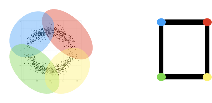
The nerve graph has four vertices, one for each of the covering sets. The vertices corresponding to the yellow and red sets are connected by an edge because they overlap. The vertices corresponding to the yellow and blue sets are not connected by an edge because they do not overlap. Building a graph representation of a dataset by constructing a good covering is a powerful technique, motivated by fundamental results like the nerve lemmas, which give guarantees about topological equivalence of a space with the nerve of a sufficiently nice cover of that space. There are numerous strategies for constructing such graph models motivated by this simple construction. Of course, the graphs constructed often have many more vertices than the model above. This kind of graph modeling is a part of an area of data science called Topological Data Analysis.
Graphical modeling can be used to understand the internals of neural networks, as illustrated below, from this paper (a presentation can be found here).
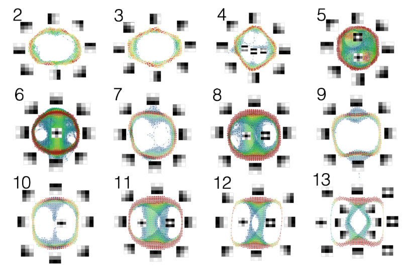
These graphs were obtained from VGG16, a convolutional neural network pre-trained on ImageNet. For each layer, we constructed the data set of weight vectors for each neuron, including only those vectors satisfying a certain local density threshold. One can see that in the first two layers, the graph model is circular, and it shows that the weight vectors are concentrated around those which detect approximations to linear gradients. Later layers always include these but also additional ones. For example, layer four includes weight vectors which detect a horizontal line against a dark background. Layer five includes a white “bulls eye” and a crossing of two lines. Later layers include combinations of these. The coloring of the nodes encodes the number of data points in the set corresponding to the node, so red points would contain more points than green or blue ones. These visualizations demonstrate the presence of geometric structure in VGG16's weight vectors, indicating that specific, interpretable features are learned at each layer.
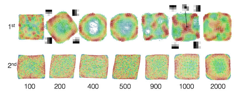
A second example performs the same kind of analysis for a two hidden layer convolutional neural network, but observing how the structure changes over the course of training. In this case, in the first layer, one can see roughly random behavior after 100 iterations, but after 200 iterations, one sees concentration (as indicated by the redness) around points on the circular boundary, which correspond to the linear gradients as in VGG16. This pattern becomes even more pronounced after 400 iterations, but begins to degrade after 500 iterations. In the second layer, one sees a very weak circular boundary through the first 500 iteration, becoming more pronounced after that. One can hypothesize that the second layer is “compensating” for the degradation occurring in the first layer. The first layer has opted to retain the linear gradients in the vertical and horizontal directions, but has additionally included a black bulls eye on a lighter background. This is unexpected behavior, and probably is due to the small number of layers in this network. What we would have expected is behavior similar to that seen in VGG16 above, in which the earliest layers respond to the simplest local behavior, namely an edge, and later layers to more complex behaviors.
III. Mechanistic Interpretability
Apollo Research recently led an extensive report on open problems in mechanistic interpretability, with a large portion focused on open questions about SAEs. Some of the issues that stood out to us were:
- As it is, the method does not create a usable geometry on the space of features. Geometry (and, we would add, topology) of feature sets is a useful way of organizing the features, and obtaining understanding and interpretations of them. It is well known that geometries of feature spaces are often extremely useful in signal processing. Fourier analysis uses the circular geometry of periodic data in a critical way, and the field of graph signal processing illustrates the power of geometry in organizing the features of a data set (see here and here for more details).
- SAEs give an organization of the activations in neural networks, level by level, but does not directly give information about mechanisms. How can one represent mechanisms?
- The ultimate goal is to extract interpretable features that accurately describe the internal processes of a model. Sparsity is used as a proxy for interpretability in SAEs. However, it is not clear whether sparsity is the best proxy for interpretability, or even always a helpful one. There are methods being developed which may improve the situation, notably minimum description length. We believe that geometrically inspired measures will yield improved interpretability.
IV. Graph Modeling of SAE features
Question 1 above concerns the need for a geometry on feature spaces. This is a key ingredient in interpretability of features. We think TDA can help understand this feature geometry, and we'll show a few simple examples we've tried on the SAE features constructed by OpenAI for GPT-2-small. The graphs we build are constructed using BluelightAI's Cobalt software, which employs a variant of the Mapper technique outlined in Section II. We did need to implement a few workarounds to make this function, and we plan to share a cleaned-up Colab notebook detailing the process in the near future. The largest component of the graph constructed on these SAE features is displayed below. We used cosine similarity to compare features.
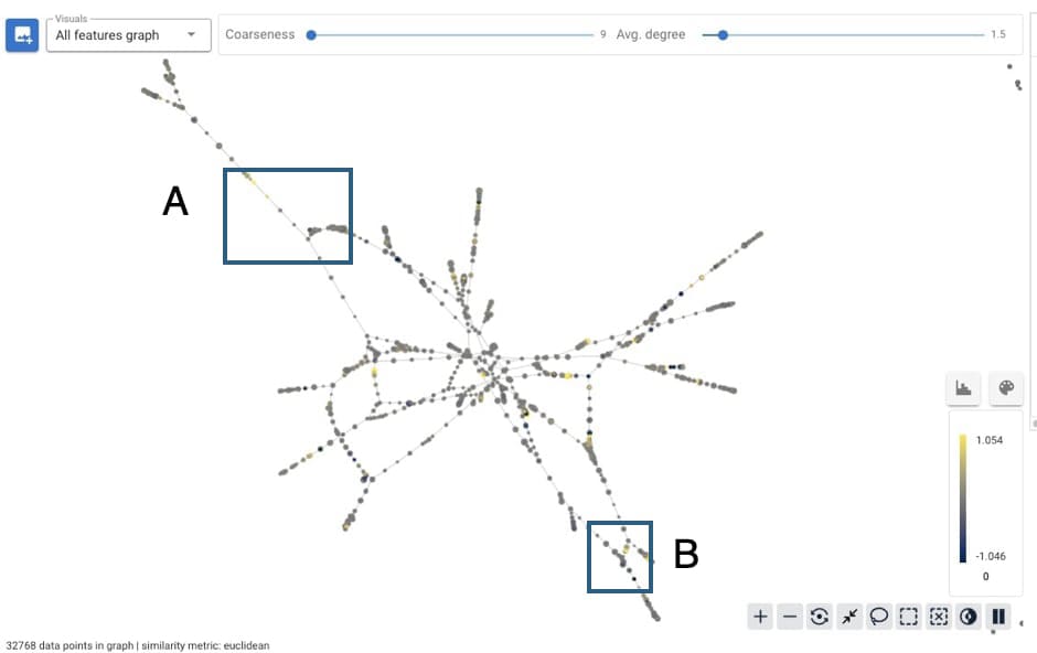
Each node of the graph corresponds to a collection of the SAE features. Below we will show selections A and B from the above diagram, and indicate what words or concepts trigger the features in each node or region. Each SAE feature activates with varying frequency on different sets of words, and collections of features are labeled by the most frequently occurring words in the collection.
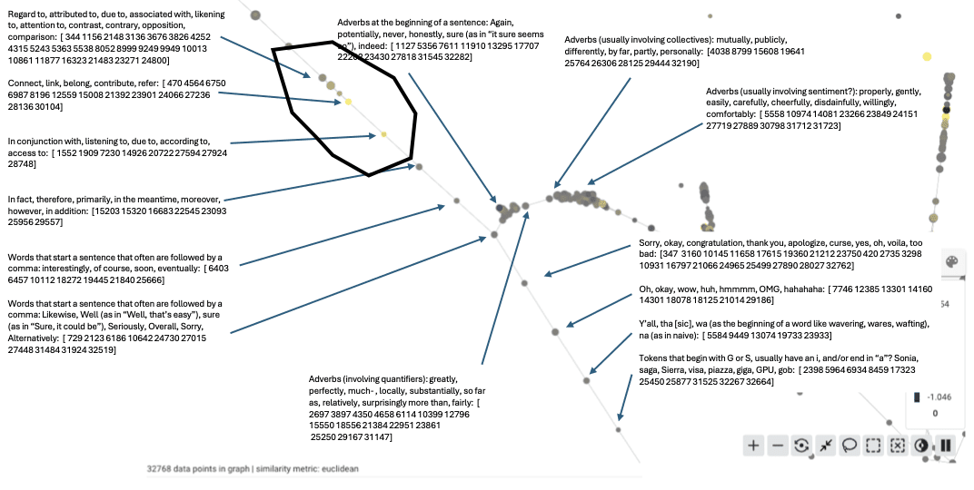
Selection A contains a three step progression, which looks like this:
(1) Regard to, attributed to, associated with, likening to
(2) Connect, link, belong, contribute, refer
(3) In conjunction with, listening to, according to, access to
All three have to do with relationships. (1) describes type of relationships, and those relationships are conceptual. (2) describes more explicit types of relationships, and (3) gives even more explicit and detailed forms of relating.
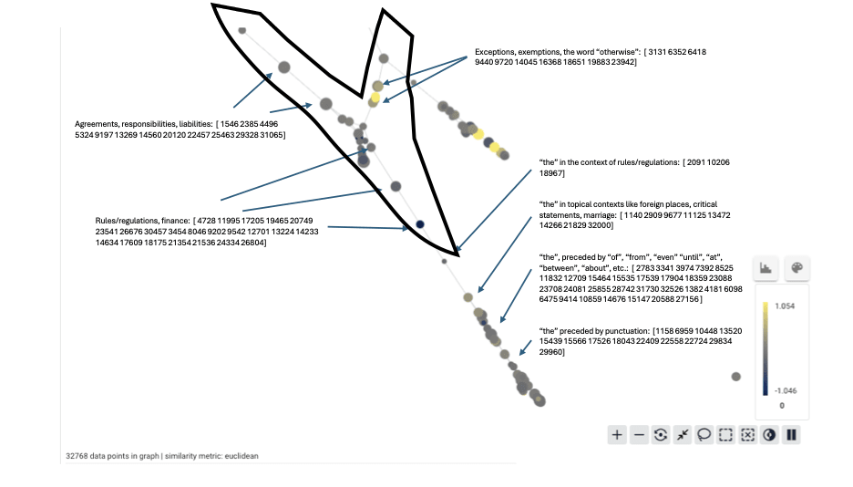
Selection B contains a “Y”-shape enclosed in the upper left, and we can interpret it like this:

V. Next steps for TDA and SAE features
We have a lot more ideas for how to use TDA to help better understand SAEs and neural network activation spaces more generally.
- What is the relationship between the geometric structure of feature decoder vectors and the geometric structure of feature activations on a corpus?
- It is possible for highly coactivating features to have dissimilar decoder vectors. Does this indicate the existence of different pathways by which the model computes similar information?
- There are TDA-based techniques that could integrate both perspectives into a single graph.
- Why are some features more densely packed in coactivation space than others?
- The features we looked at above were found in the densest region of the data
- Is there interesting topological structure in the less-dense regions of feature space?
- What is the best way to extract a relevant subset of features to explore from a large feature library?
- We can build graphs on large sets of features, but it can be hard to visually navigate such large graphs.
- If we want to explore feature activations on a particular input, is it useful to “zoom in” on a neighborhood of the highly activating features for that input?
- What do the relationships between features in different layers of a model look like from a TDA perspective?
- We can build graphs on both feature sets, and implement an interactive exploration where selecting nodes in one graph colors the other to highlight things like co-occurring features.
We looked at the geometric structure of SAE features themselves here, but we think these features may also be useful as a way to better understand the topological structure of activation space:
- Are some SAE features only contextually relevant? Does this lead to understanding SAE features as coordinates for something like local charts of an activation manifold?
- Can we see contextual features as working like a fiber bundle or sheaf over a space of more globally-relevant features?
- What does a topological analysis of the SAE reconstruction residual look like? Is there any signal in the data that might indicate the types of information that SAEs find hard to capture?
VI. Summary
We have demonstrated the use of topological data analysis in the study of SAEs for large language models, and obtained conceptual understanding of groups of these features. This methodology is quite powerful, and holds the promise for the mechanistic understanding of the internals of large language models.
VII. Acknowledgments
We thank Lee Sharkey for his helpful comments and suggestions.
4 comments
Comments sorted by top scores.
comment by Jakob Hansen · 2025-02-25T22:16:38.255Z · LW(p) · GW(p)
Here is the promised Colab notebook for exploring SAE features with TDA. It works on the top-k GPT2-small SAEs by default, but should be pretty easily adaptable to most SAEs available in sae_lens. The graphs will look a little different from the ones shown in the post because they are constructed directly from the decoder weight vectors rather than from feature correlations across a corpus.
One of the interesting things I found while putting this together is a large group of "previous token" features, which are mostly misinterpreted by the LLM-generated explanations. These have been noted in attention SAEs (e.g. https://www.alignmentforum.org/posts/xmegeW5mqiBsvoaim/we-inspected-every-head-in-gpt-2-small-using-saes-so-you-don [AF · GW]), but I haven't seen much discussion of them, although they seem very relevant for implementing induction heads. The fact that they are grouped together in the graph makes sense if they are all computed by or used as the input to a single attention head, or more generally if there is some subspace of the residual stream reserved for this kind of information, although I haven't yet checked if this is the case.
comment by Martin Vlach (martin-vlach) · 2025-03-07T07:17:46.649Z · LW(p) · GW(p)
No matter how I stretch or compress the digit 0, I can never achieve the two loops that are present in the digit 8.
0 when it's deformed by left and right pressure so that the sides meet seems to contradict?
Replies from: gunnar-carlsson↑ comment by Gunnar Carlsson (gunnar-carlsson) · 2025-03-10T20:29:00.064Z · LW(p) · GW(p)
Sorry, did not make the notion of deformation precise. The idea is that stretching and compressing cannot include attaching one part to another, or tearing it. The mathematical term is that of a "homeomorphism" , which is a one to one, onto, and continuous map. The precise statement is that the figure 8 is not homeomorphic to zero. A good place to look is
https://www.google.com/books/edition/Basic_Topology/NJbuBwAAQBAJ?hl=en&gbpv=1&printsec=frontcover
Replies from: martin-vlach↑ comment by Martin Vlach (martin-vlach) · 2025-03-11T17:43:51.004Z · LW(p) · GW(p)
Yeah, I've met the concept during my studies and was rather teasing for getting a great popular, easy to grasp, explanation which would also fit the definition.
It's not easy to find a fitting visual analogy TBH, which I'd find generally useful as I hold the concept to enhance general thinking.