PaLM-2 & GPT-4 in "Extrapolating GPT-N performance"

post by Lukas Finnveden (Lanrian) · 2023-05-30T18:33:40.765Z · LW · GW · 6 comments

Contents

  Converting to Chinchilla scaling laws
  PaLM-2
  GPT-4
  Appendix — How I convert to Chinchilla loss
None
6 comments

Two and a half years ago, I wrote Extrapolating GPT-N performance [LW · GW], trying to predict how fast scaled-up models would improve on a few benchmarks. One year ago, I added PaLM to the graphs [LW · GW]. Another spring has come and gone, and there are new models to add to the graphs: PaLM-2 and GPT-4. (Though I only know GPT-4's performance on a small handful of benchmarks.)

Converting to Chinchilla scaling laws

In previous iterations of the graph, the x-position represented the loss on GPT-3's validation set, and the x-axis was annotated with estimates of size+data that you'd need to achieve that loss according to the Kaplan scaling laws. (When adding PaLM to the graph, I estimated its loss using those same Kaplan scaling laws.)

In these new iterations, the x-position instead represents an estimate of (reducible) loss according to the Chinchilla scaling laws. Even without adding any new data-points, this predicts faster progress, since the Chinchilla scaling laws describes how to get better performance for less compute.

The appendix describes how I estimate Chinchilla reducible loss for GPT-3 and PaLM-1. Briefly: For the GPT-3 data points, I convert from loss reported in the GPT-3 paper, to the minimum of parameters and tokens you'd need to achieve that loss according to Kaplan scaling laws, and then plug those numbers of parameters and tokens into the Chinchilla loss function. For PaLM-1, I straightforwardly put its parameter- and token-count into the Chinchilla loss function.

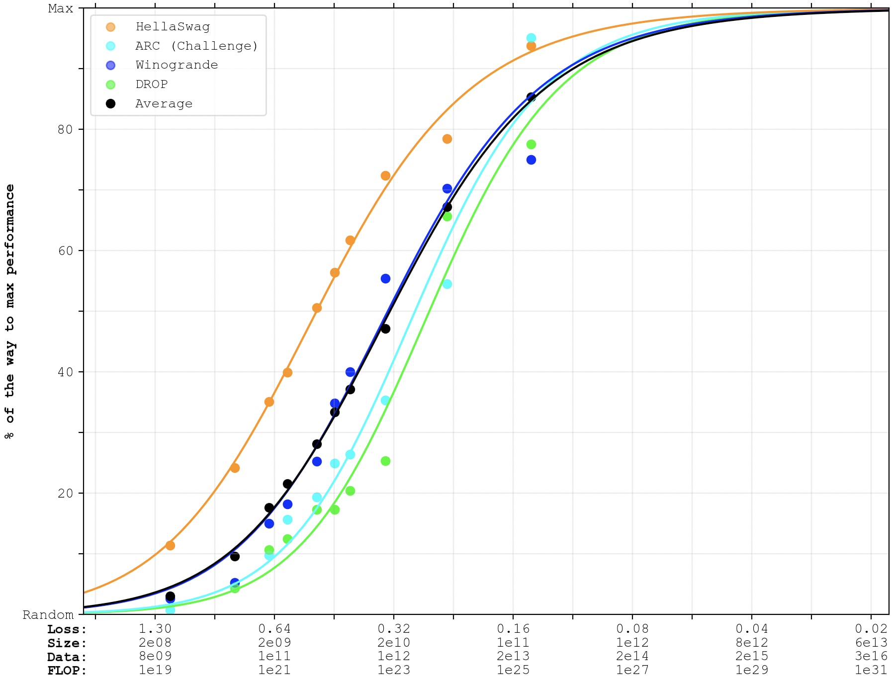
To start off, let's look at a graph with only GPT-3 and PaLM-1, with a Chinchilla x-axis.

Here's a quick explainer of how to read the graphs (the original post [LW · GW] contains more details). Each dot represents a particular model’s performance on a particular category of benchmarks (taken from papers about GPT-3 and PaLM). Color represents benchmark; y-position represents benchmark performance (normalized between random and my guess of maximum possible performance).

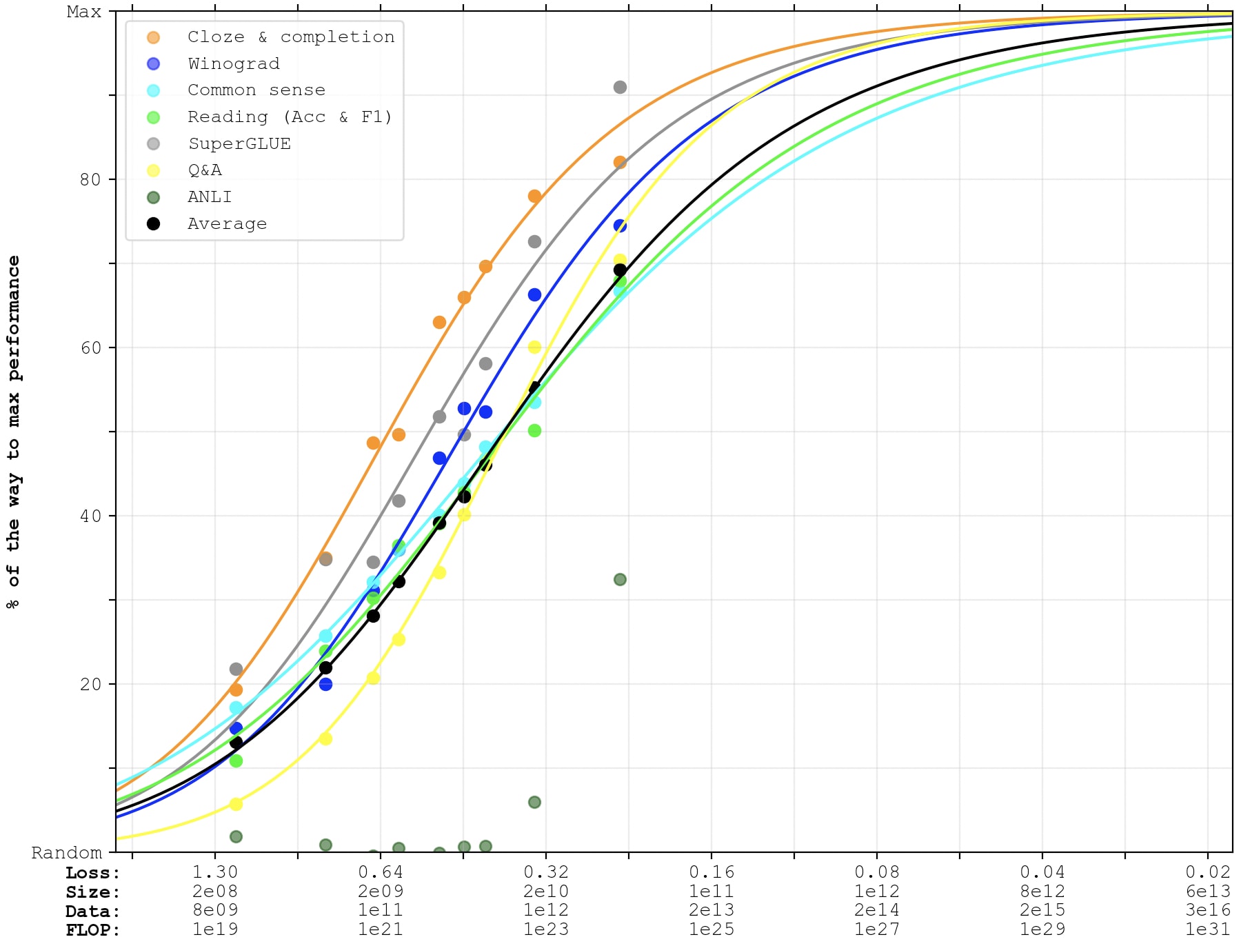
The x-axis labels are all using the Chinchilla scaling laws to predict reducible loss-per-token, number of parameters, number of tokens, and total FLOP (if language models at that loss were trained Chinchilla-optimally).

Compare to the last graph in this comment [LW(p) · GW(p)], which is the same with a Kaplan x-axis. Some things worth noting:

• PaLM is now ~0.5 OOM of compute less far along the x-axis. This corresponds to the fact that you could get PaLM for cheaper if you used optimal parameter- and data-scaling.
• The smaller GPT-3 models are farther to the right on the x-axis. I think this is mainly because the x-axis in my previous post had a different interpretation.^[1]
• The overall effect is that the data points get compressed together, and the slope becomes steeper. Previously, the black "Average" sigmoid reached 90% at ~1e28 FLOP. Now it looks like it reaches 90% at ~5e26 FLOP.

Let's move on to PaLM-2. If you want to guess whether PaLM-2 and GPT-4 will underperform or outperform extrapolations, now might be a good time to think about that.

PaLM-2

If this CNBC leak is to be trusted, PaLM-2 uses 340B parameters and is trained on 3.6T tokens. That's more parameters and less tokens than is recommended by the Chinchilla training laws. Possible explanations include:

• The model isn't dense. Perhaps it implements some type of mixture-of-experts situation that means that its effective parameter-count is smaller.
• It's trained Chinchilla-optimally for multiple epochs on a 3.6T token dataset.
• The leak is wrong.

If we assume that the leak isn't too wrong, I think that fairly safe bounds for PaLM-2's Chinchilla-equivalent compute is:

• It's as good as a dense Chinchilla-optimal model trained on just 3.6T tokens, i.e. one with 3.6T/20=180B parameters. This would make it 6*180e9*3.6e12=3.9e24 FLOP.
• It's as good as a dense Chinchilla-optimal model with 340B parameters, i.e. one that was trained with 20*340B=6.8T tokens. 6*340e9*6.8e12=1.4e25 FLOP.

So I'll talk about both of those.

The PaLM-2 technical report reports 1-shot performance instead of few-shot performance, which my previous posts focused on (and which is depicted in the above graph). So the following graphs will display 1-shot performance from both GPT-3 and PaLM. Performance will be generally lower.

First, how well does PaLM-2 match up against what you would have predicted from looking at GPT-3 and PaLM-1? In the following graph:

• The dots are GPT-3 and PaLM-1 data points. The lines are only fit to the dots.
• The first line of crosses is the smaller estimate for PaLM-2: 3.9e24 FLOP.
• The second line of crosses is the larger estimate for PaLM-2: 1.4e25 FLOP.

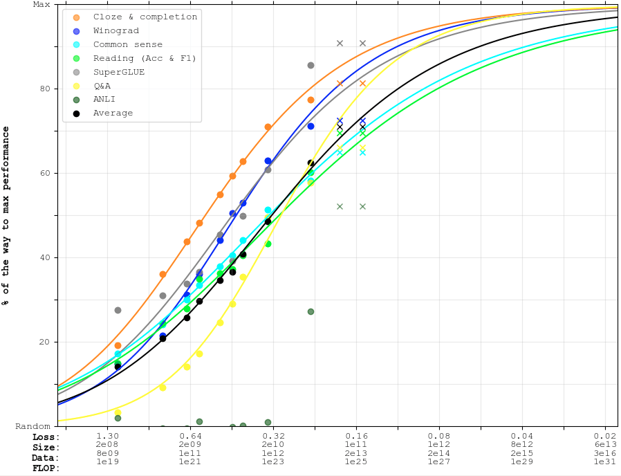
As it so happens, my reflections from last year (when adding PaLM to just the GPT-3 points) apply ~equally well for PaLM-2:

• SuperGLUE is above trend. ANLI sees impressive gains, though nothing too surprising given ~sigmoidal scaling.
• Common sense reasoning + Reading tasks are right on trend.
• Cloze & completion, Winograd, and Q&A are below trend.
• The average is amusingly right-on-trend, though I wouldn’t put a lot of weight on that, given that the weighting of the different benchmarks is totally arbitrary.
  • (The current set-up gives equal weight to everything — despite e.g. SuperGLUE being a much more robust benchmark than Winograd.)

Maybe this is because the lines are still dominated by all the GPT-3 data points (despite also being fit to PaLM-1), and because PaLM-2 is pretty similar to PaLM.

This graph doesn't really help us tell whether PaLM-2 was trained with ~3.9e24 FLOP-equivalent or ~1.4e25 FLOP-equivalent. The average trend is slightly below the former and slightly above the latter.

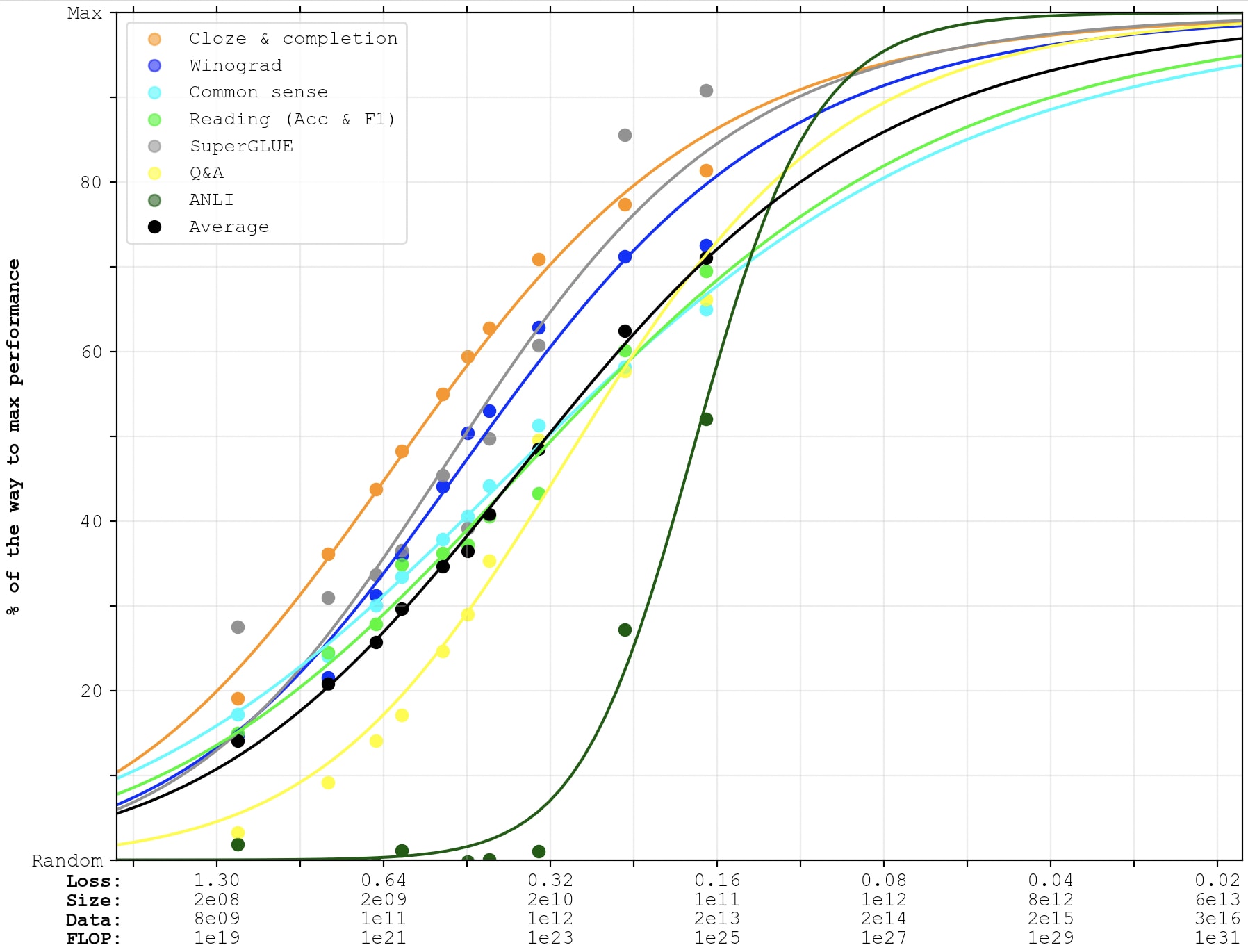
So for fitting sigmoids to the PaLM-2 data points (along with the other data points, for future extrapolations), I'll split the difference and pretend that their 340B parameters trained on 3.6T tokens was equally good as a Chinchilla-optimal training-run with the same compute-budget: 6*340e9*3.6e12=7.3e24 FLOP.

GPT-4

For GPT-4's x-position, I'll use Epoch's estimate of 2e25 FLOP, and assume that GPT-4 is equally good as a Chinchilla-optimal model trained with that much compute would be.

Unfortunately, the GPT-4 technical report only reports performance on 4 out of the >20 benchmarks that I've been using previously. So the following graph will have fewer lines, and each line will only represent a single benchmark (and therefore be noisier). As above, I've fit the lines to GPT-3 as well as PaLM-1, and the crosses represent GPT-4. (PaLM-2 is no longer included in the graph, since they don't report few-shot performance on all of these benchmarks, which is what we're looking at now.)

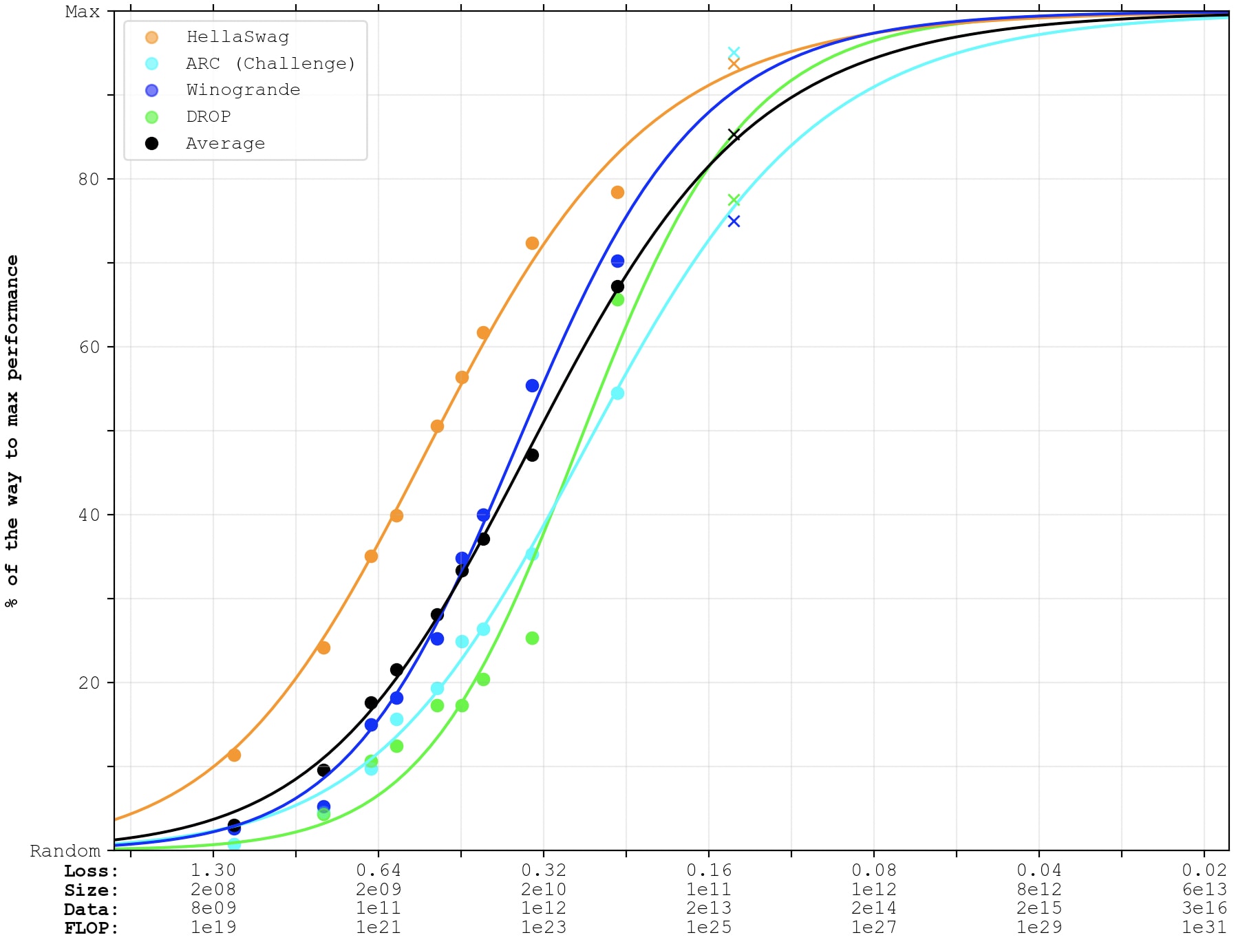
GPT-4 outperforms expectations on ARC (AI2 Reasoning Challenge, challenge-set), which is grade-school multiple-choice science-questions.

GPT-4 underperforms expectations on WinoGrande (commonsense reasoning around pronoun resolution) and  DROP (reading comprehension & arithmetic).

GPT-4 performs as-expected on HellaSwag (commonsense reasoning around everyday events).

It's average performance is right-on-trend. I think I would have expected GPT-4 to be better than 2e25-FLOP-equivalent, given algorithmic improvements and fine-tuning. So maybe a small amount under-trend. (Compared to this very noisy extrapolation of 4 almost-saturated benchmarks.)

Here's a graph where the sigmoids are also fit to the GPT-4 data points:

Appendix — How I convert to Chinchilla loss

The obvious way to estimate models' Chinchilla-equivalent loss would be to take the number of parameters (N) and the number of tokens (D) that were used to train each model and plug them into the Chinchilla scaling law: reducible loss = 406.4*N^(-0.34) + 410.7*D^(-0.28).

This is indeed what I do for PaLM-1.

But this would probably overestimate performance for the smaller GPT-3 models. All models in the GPT-3 paper were trained on the same 300B tokens, which is much more than what the Kaplan scaling laws recommend. This would boost Chinchilla-estimated performance by a fair bit. But those models probably didn't have the right hyperparameters to make use of all that data. (My impression is that Kaplan et al. estimated the wrong scaling laws because they were using suboptimal hyperparameters.)

I'll instead do a somewhat more complicated thing, where I estimate Chinchilla-equivalent loss as follows:

• I start from the empirical loss that each model in the GPT-3 paper is reported to have on their validation set.
• I then use the scaling law from Figure 3.1 of the GPT-3 paper to estimate a Kaplan-equivalent compute. L = 2.57*C^(-0.048) <-> C = (L/2.57)^(-1/0.048).
• I then use the scaling laws from equation B.9 in appendix B of the Kaplan scaling law paper to compute Kaplan-optimal number of tokens and parameters to use if you're training a model with that much compute.
  • There are multiple different scaling laws you could get from that paper, which says different things. I choose B.9 because it has the closest match to the parameters and tokens that the largest version of GPT-3 actually has. (It says that a model with GPT-3's compute should have had 164B parameters and 319B tokens rather than 175B and 300B.)
• I then use the Chinchilla law L = 406.4*N^(-0.34) + 410.7*D^(-0.28) to estimate how much loss a model like that would have gotten on Chinchilla's validation set.
• And I use the Chinchilla scaling laws to estimate the minimum number of compute you'd need to achieve that loss — and what split of parameters and data you should use.

The key assumptions that this relies on is (i) the accuracy of the B.9 scaling law for the way that the Kaplan authors were training models, and (ii) that the Kaplan authors and the Chinchilla authors were ~equally good at training capable models when the param/token-split was as-recommended by Kaplan.

Here's a figure over how this way of doing things correspond to mapping directly from parameters and data. Each dot is a model described in the GPT-3 paper. Their x- and y-positions represent (the logarithm of) the estimated FLOP needed to train a Chinchilla-optimal model with that level of performance, according to the two different methodologies.

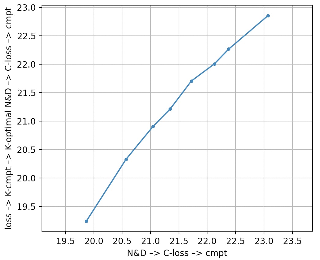
In the middle, the two methodologies are briefly ~equivalent (the line almost goes through (21.5,21.5)). At the lower end, the two methodologies differ by a factor of ~4. At the top end (GPT-3 itself), they differ by a factor ~1.6.

1. ^{^}

   Previously, the "Data" annotations represented how much data you'd need to reach a certain level of performance (for the given model-size) if you trained until convergence on that data, for as many epochs as was needed. On this new graph, the "Data" annotation instead represents the total number of tokens you train on (only for a single epoch) — which means that the numbers are larger.

   Why the discrepancy? Due to some "contradictions" in the Kaplan scaling laws (see my original post for more details), it was known that current compute-optimal scaling couldn't keep working for much longer. It looked more likely that the "train until convergence"-scaling laws would remain accurate. Furthermore, Kaplan scaling laws recommended training on fewer and fewer epochs as you scaled model-size, so in the near future, it seemed likely that models would converge in ~1 epoch. This meant that I could estimate future compute-budgets as 6*#parameters*#tokens with #parameters and #tokens estimated using the "train until convergence"-scaling laws.

6 comments

Comments sorted by top scores.