Toy Models of Superposition: Simplified by Hand
post by Axel Sorensen (axel-sorensen) · 2024-09-29T21:19:52.475Z · LW · GW · 3 commentsContents
  Introduction
  Superposition: A simple example
  What do the embeddings mean?
  Superposition: By Hand
    Preserve first and second feature
    Embed all three features with interference
    Importance and embeddings
  Adding the bias vector
    Perfectly reconstruct one example
    Cancelling out interference
  Adding the ReLU activation function
  Try it yourself
  Closing remarks
None
3 comments
Introduction
In Anthropic's paper "Toy Models of Superposition", they illustrate how neural networks represent more features than they have dimensions by embedding them in so-called "superposition". This allows the model to represent more information (although at the cost of interference) and leads to polysemantic neurons (that correspond to multiple features).
When I first read the paper, I struggled to intuitively grasp what the embeddings in superposition actually represented and what interference between features concretely looked like. In this post, I aim to break down the concept of superposition by hand and provide a simple walkthrough of the underlying "machinery".
I must confess that I am relatively new to the field of mechanistic interpretability and I warmly welcome any thoughts, suggestions, or corrections on my interpretations.
Let's begin with a refresher on superposition.
Superposition: A simple example
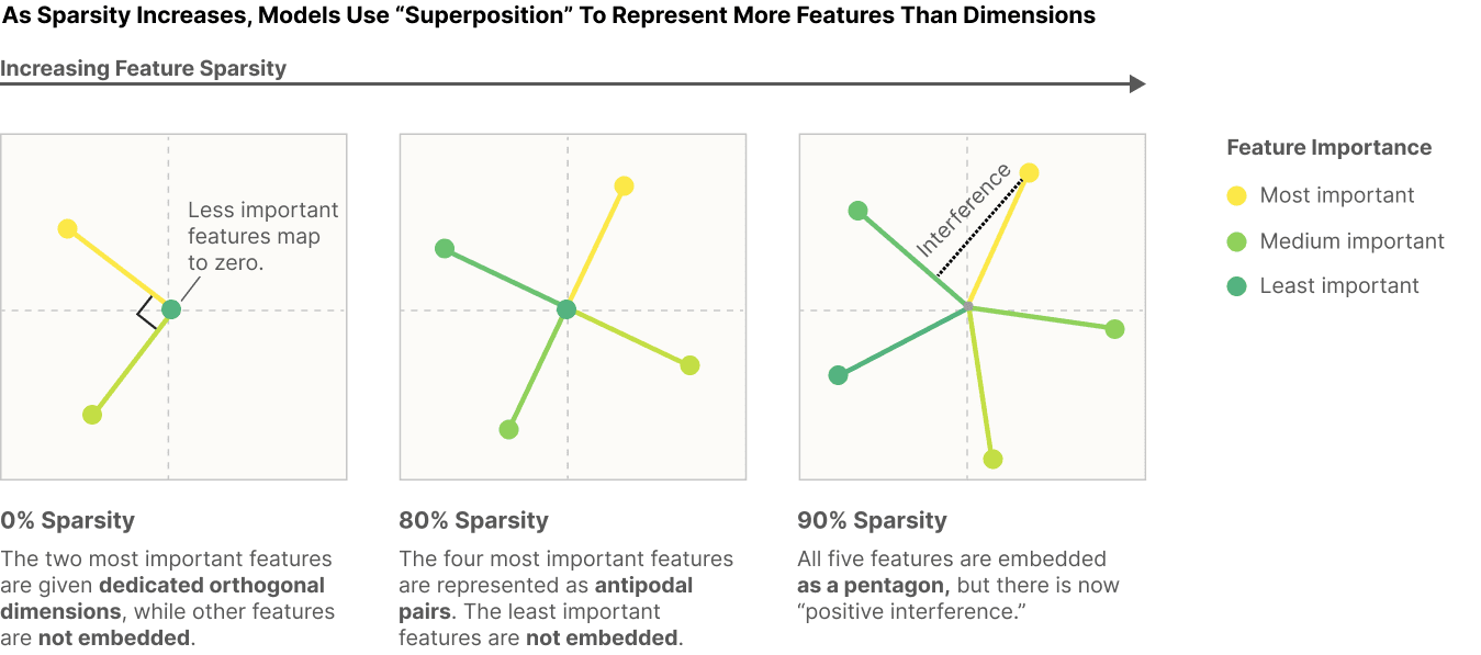
When features are sparse (meaning that they rarely co-occur), superposition becomes an attractive strategy. The authors illustrate this with a simple example. Consider a toy model trained to embed five features of varying importance in two dimensions (see Figure 1). In this case, the training data (of size N) is generated by sampling 5 random numbers N times from a uniform distribution. Feature sparsity determines how likely it is for each feature in a data point to be zero.

What do the features represent?
In image or text data, features are usually not explicitly specified. However, if certain patterns or characteristics of the input data are useful for the task at hand, a model may learn to represent the presence of these "features".
In our case, we skip a step and artificially populate the activations of each of these features. For example, the input to our model might look like this:
When features always co-occur (0% sparsity), the model learns to represent an orthogonal basis of the most important two features while ignoring the rest. As feature sparsity increases, the model gradually embeds more features until all five features are embedded in superposition at the cost of interference between the embeddings.
But what do the embeddings mean and where do they come from?
What do the embeddings mean?
In the toy example, the model is tasked with projecting five features onto two dimensions and then reconstructing the features from this embedding. The vectors in Figure 1 represent the 5 by 2 weight matrix that projects the five features into 2D space. The model's loss is defined as the square error between the feature and its reconstruction. This incentivizes the model to learn an embedding that minimizes the overall reconstruction loss.
In the authors' example, each feature is assigned a different importance, weighting how much it contributes to the overall loss.
What is importance?
Not all features are equally useful for a given task. When learning to classify different dog breeds, a 'floppy ear' feature might be more important than a 'grass' feature. This, in turn, means that not representing 'floppy ears' will have a greater impact on the loss than not representing 'grass'.
The importance of a feature is artificially introduced by weighting the error between each feature and its reconstruction with the corresponding importance value.
The output of the model (the reconstruction of the features from 2D space) is calculated as follows. The model receives a vector x of N features. This vector is multiplied by a weight matrix W of shape N x D, where D is the dimension of the embedding space.
The output of this multiplication is then multiplied by the transpose of the weight matrix.
Finally, a bias vector b is added to the output (1 bias per feature) and the result is passed through a ReLU activation function.
Written out in full:
Superposition: By Hand
In order to understand exactly what is going on, let us explore the model by hand. Imagine an even simpler example; Three features represented in two dimensions. We define the feature vector as follows:
The weight matrix must then be a 3 by 2 matrix. Let us forget about the bias vector and ReLU function for now and focus only on the projection and reconstruction of the features:
Since we are compressing 3 numbers into 2 numbers, it is not possible to retain all of the initial information.
Preserve first and second feature
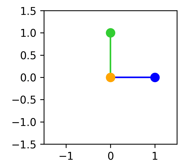
We may choose to preserve the exact values of the first and second features while ignoring the third. In this case, the weight matrix would look as follows:
Plotting the embeddings would look like this: (Feature 1 = blue, feature 2 = green, feature 3 = orange)

When projecting our features into 2D space we get:
And when reconstructing them again we end up with:
The first and second features are perfectly reconstructed while the third is completely lost. Since the embedding of the first feature ([1,0]) and the embedding of the second feature ([0,1]) are orthogonal. No interference happens between them.
Embed all three features with interference
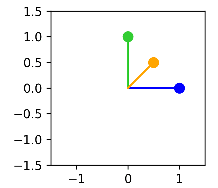
We may also choose to embed all three features at the cost of interference. In this case, the weight matrix could look as follows:
Plotting the embeddings would look like this: (Feature 1 = blue, feature 2 = green, feature 3 = orange)

When projecting our features into 2D space we get:
And when reconstructing them again we end up with:
Now information from the third feature is reconstructed, however positive interference occurs between the features, adding a bit of noise to each value in the reconstruction. There is still no interference between the first and the second feature (since they are orthogonally embedded), however, the third feature interferes with and receives interference from the first and second feature.
Importance and embeddings
Imagine that one of the features is more important than the others in regards to the model loss. This would mean that an error in the reconstruction of this feature would contribute more to the loss than that of the other features, incentivizing us to reconstruct this feature perfectly (at the potential cost of less accurate reconstructions of the rest)
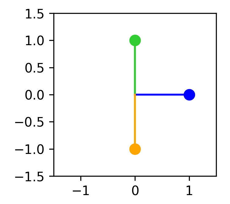
Let's say feature 1 is more important. Then we may want to represent it orthogonally to the second and third features. The only way to do this is by embedding the second and third features in an antipodal structure, resulting in the following weight matrix:
Plotting the embeddings would look like this: (Feature 1 = blue, feature 2 = green, feature 3 = orange)

When projecting our features into 2D space we get:
And when reconstructing them again we end up with:
Now the first feature is perfectly reconstructed, however at the cost of severe negative interference between the second and third feature.
Adding the bias vector
Without a bias vector, it is not possible to embed all three features in 2D space without at least some interference. However, the bias vector may help with that. Remember that we add the bias vector like this.
Perfectly reconstruct one example
If we know the values beforehand we can simply represent the first and second features.
Project:
Reconstruct:
And now simply add the third feature in through the bias, to end up with a perfect reconstruction.
Of course, knowing the values beforehand is hardly ever the case and this strategy would not work for varying inputs. Instead, the bias vector can be useful for canceling out noise introduced by the interference.
Cancelling out interference
In a previous example, we embedded the second and third features in an antipodal structure. This resulted in severe interference between the two features and an inaccurate reconstruction. Let us see how the bias vector can help with that.
When projecting our features into 2D space we get:
And when reconstructing them again we end up with:
We know that the presence of the second feature will shrink the value of the reconstruction of the third feature, but we don't know how much (since this depends on the value of the second feature). Let us go with the expected value of the uniform distribution between 0 and 1; 0.5. We don't add any bias value to the first feature since this feature is orthogonal to the second and third (thereby not receiving any interference). But we add 0.5 to the reconstruction of the second and third features, partially mitigating the negative interference. This results in the following vector.
We still don't have a perfect reconstruction, but the output is much closer to the original features than before.
Adding the ReLU activation function
The ReLU activation function is not necessary for embedding features in superposition, however, it's non-linear properties are helpful to cancel out negative interference when only 1 feature is present.
Imagine we have learned the same embeddings as in the previous example but a new input comes in:
When projecting our features into 2D space we get:
And when reconstructing them again we end up with:
Now we pass the output through the ReLU, setting all negative values to zero:
This perfectly reconstructs the original features. In this way, the ReLU function makes negative interference 'free' when there's only one feature present at a time.
Try it yourself
Now it's time for you to give it a shot
Given an input of three features:
What would the weight matrix and bias vector have to be to output a perfect reconstruction? (Note: There is no unique answer)
Possible answers
If we choose to just add in the 3rd feature through the bias vector we might define the following:
Another possible solution could be:
First we project:
Then we reconstruct:
And finally add the bias term:
The ReLU doesn't change the output:
So far we have only seen examples where we are trying to embed a particular input. If we were machine learning algorithms this would be referred to as overfitting. The goal is to find an embedding that works well for several different inputs. Depending on the sparsity of features (the probability of a feature being zero) some embeddings might be more advantageous than others.
What would the weight matrix and bias vector look like for a solution that would generalize to random features (each feature sampled from a uniform distribution between 0 and 1)? And how do these embeddings change as feature sparsity increases?
I will leave this as an exercise for the reader.
Closing remarks
I hope this short explainer made the embeddings behind superposition a bit more tangible. I learned a lot by going through the embedding by hand and thinking about the balance between reconstruction loss and interference. As well as the role of the bias vector and the ReLU function in adjusting the output.
Feel free to leave your thoughts, solutions, and observations in the comments or reach out at axelsorensenwork@gmail.com. And let me know if there might be other concepts that could benefit from a "Simplified by Hand" edition.
3 comments
Comments sorted by top scores.
comment by Martin Vlach (martin-vlach) · 2024-10-17T13:59:43.064Z · LW(p) · GW(p)
I have not read your explainer yet, but I've noted the title Toy Models of Superposition: Simplified by Hand [LW · GW] is a bit misleading in the sense to promise to talk about Toy Models which it is not at all, the article is about Superposition only, which is great but not what I'd expect looking at the title.
Replies from: axel-sorensen↑ comment by Axel Sorensen (axel-sorensen) · 2024-10-21T14:37:22.531Z · LW(p) · GW(p)
Hey Martin
Thanks for your input, it was not my intention to be misleading.
When you say "the article is about Superposition only" are you referring to my post or the original article by Anthropic? Since they named their article "Toy Models of Superposition" and my post is heavily based on the findings in that paper, I choose the title to serve as a pointer towards that reference. Especially because I could've used a visual pen and paper breakdown when I originally read that very article.
Feel free to read my explainer and suggest a better title :)
↑ comment by Martin Vlach (martin-vlach) · 2024-10-31T16:26:41.596Z · LW(p) · GW(p)
I mean your article, Anthropic's work seems more like a paper. Maybe without the ": S" it would make more sense as the reference and not a title: subtitle notion.