Learning coefficient estimation: the details

post by Zach Furman (zfurman) · 2023-11-16T03:19:09.013Z · LW · GW · 0 comments

This is a link post for https://colab.research.google.com/github/zfurman56/intro-lc-estimation/blob/main/Intro_to_LC_estimation.ipynb

Contents

  What this is for
  What this isn't for
  TLDR 
None
No comments

What this is for

The learning coefficient (LC), or RLCT, is a quantity from singular learning theory that can help to quantify the "complexity" of deep learning models, among other things.

This guide is primarily intended to help people interested in improving learning coefficient estimation get up to speed with how it works, behind the scenes. If you're just trying to use the LC for your own project, you can just use the library without knowing all the details, though this guide might still be helpful. It's highly recommended you read this post [LW · GW] before reading this one, if you haven't already.

We're primarily covering the WBIC paper (Watanabe 2010), the foundation for current LC estimation techniques, but the presentation here is original, aiming for better intuition, and differs substantially from the paper. We'll also briefly cover Lau et al. 2023.

Despite all the lengthy talk, what you end up doing in practice is really simple, and the code is designed to highlight that. After some relatively quick setup, the actual LC calculation can be comfortably done in one or two lines of code.

What this isn't for

• A good overview of SLT, or motivation behind studying the LC or loss landscape volume in the first place. We're narrowly focused on LC estimation here.
• Sampling details. These are very important! But they're not really unique to singular learning theory, and there are plenty of good resources and tutorials on MCMC elsewhere.
• Derivations of formulas, beyond the high-level reasoning.

TLDR 

• What is the learning coefficient? (Review from last time [LW · GW])
  • The learning coefficient (LC), also called the RLCT, measures basin broadness.
  • This isn't new, but typically "basin broadness" is operationalized as "basin flatness" - that is, via the determinant of the Hessian. When the model is singular (eigenvalues of the Hessian are zero), this is a bad idea.
  • The LC operationalizes "basin broadness" as the (low-loss asymptotic) volume scaling exponent. This ends up being the right thing to measure, as justified by singular learning theory.
•  How do we measure it?
  •  It turns out that measuring high-dimensional volume directly is hard. We don't do this.
  • Instead we use MCMC to do what's known in statistics as "method of moments" estimation. We contrive a distribution with the LC as a population parameter, sample from that distribution and calculate one of its moments, and solve for the LC.
  • We simplify some details in this section, but this is the conceptual heart of LC estimation.
• How do we measure it (for real)?
  • The above is a bit simplified. The LC does measure loss volume scaling, but the "loss" it uses is the average or "infinite-data" limit of the empirical loss function.
  • In practice, you don't know this infinite-data loss function. Luckily, you already have a good estimate of it - your empirical loss function. Unluckily, this estimate isn't perfect - it can have some noise. And it turns out this noise is actually worst in the place you least want it.
  • But it all works out in the end! You actually just need to make one small modification to the "idealized" algorithm, and things work fine. This gets you an algorithm that really works in practice!
  • Finally, the state-of-the-art method (Lau et al. 2023) makes a couple simple modifications, for scalability among other reasons: it measures the learning coefficient only *locally*, and uses mini-batch loss instead of full-batch.

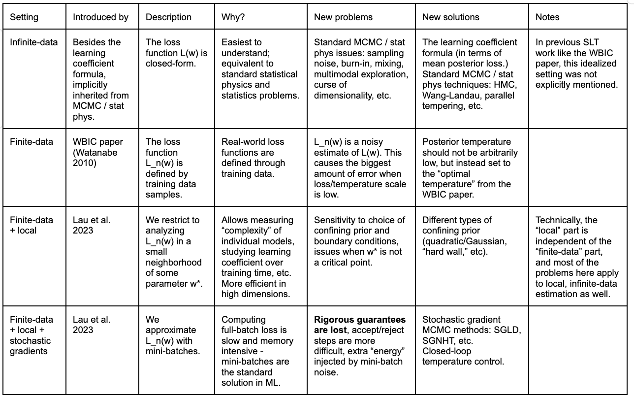
In chart form: as we move from idealized (top) to realistic (bottom), we get new problems, solutions, and directions for improvement. The guide itself covers the first two rows in the most detail, which are likely the most conceptually difficult to think about, and skips directly from the second row to the fourth row at the very end.

 

See the linked Colab notebook for the full guide.

0 comments

Comments sorted by top scores.