You’re Measuring Model Complexity Wrong
post by Jesse Hoogland (jhoogland), Stan van Wingerden (stan-van-wingerden) · 2023-10-11T11:46:12.466Z · LW · GW · 17 commentsContents
  Why Model Complexity?
    Model Comparison
    Model Development
  From Basins to Model Complexity
    Intractable: Basin Volume
    Wrong: Basin Flatness
    Instead: Basin Dimension
  Estimating Learning Coefficients
    Deriving the Estimator
    The Local Learning Coefficient
    Implementing the Estimator
    Limitations
  What's Next
None
17 comments
TLDR: We explain why you should care about model complexity, why the local learning coefficient is arguably the correct measure of model complexity, and how to estimate its value.
In particular, we review a new set of estimation techniques introduced by Lau et al. (2023). These techniques are foundational to the Developmental Interpretability research agenda [LW · GW] and constitute the first generation of methods for detecting and understanding phase transitions, with potential applications for both interpretability and mechanistic anomaly detection. We expect this set of techniques to become a fixture in the alignment toolkit, and we've published a library and examples to help you get started.
This post is based on the paper, "Quantifying degeneracy in singular models via the learning coefficient" by Edmund Lau, Daniel Murfet, and Susan Wei (2023). The content builds on previous posts by @Liam Carroll [LW · GW] on effective dimensionality in neural networks [LW · GW] and the resulting perspective on phase transitions [LW · GW].
Why Model Complexity?
Model Comparison
Comparing models matters for safety. Given two models with the same behavior on a particular set of evals, we would like to be able to predict how they'll behave on out-of-distribution data. Can we distinguish the deceptively aligned model from the non-deceptively aligned model? As a first pass, can we predict that two models will or will not behave similarly in the future?
Comparing via weights. Because models are singular (parameters do not correspond one-to-one with functions), it's not possible to compare weights directly. Very different choices of weights can implement the same functions, and very similar choices of weights can implement qualitatively different functions.
Comparing via behavior. We also can't compare models at the level of the loss because different functions are compatible with the same loss. The same is true even if we compare models sample-by-sample: we'd need an astronomical number of inputs to meaningfully constrain behavior (some of which we'd rather not expose our model to).
Comparing via invariants. Another option is to take a pointer from the mathematicians and physicists: in classifying mathematical objects like spaces, it helps to turn geometric problems into algebraic problems where we can compute invariants. If two spaces have different values of that invariant, then we know that they're different. If the values are the same, the results are inconclusive.
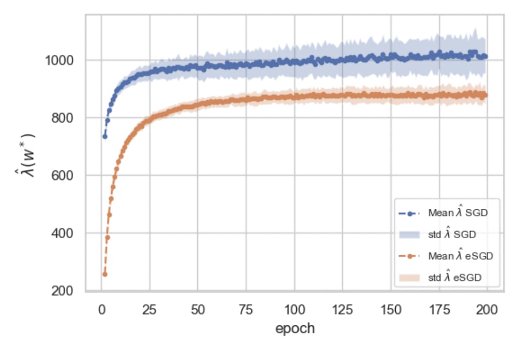
The local learning coefficient. The quantity we'll look at in this post, the (local) learning coefficient , is an invariant that measures model complexity — a coarse-grained feature of the model that is useful for making high-level comparisons with other models. Though having identical learning coefficients doesn't imply that two models are the same, having different learning coefficients tells us that two models are qualitatively different.
The learning coefficient is unique in that it is an output of the theory rather than an ad-hoc invention. Except for the loss itself, the learning coefficient is the most principled way to compare different models.
Model Development
Model comparison is necessary to study model development. We're interested in comparing models across time to understand how they develop [LW · GW]. High-level observables like the local learning coefficient give us insight into this process without requiring a detailed understanding of the model's internal mechanisms.
In particular, we're aiming to understand phase transitions during learning — moments in which models go through sudden, unanticipated shifts. We want to be able to detect these transitions because we think most of the risk is contained in sudden, undesired changes to values or capabilities that occur during training (~sharp left turns) and sudden, undesired changes to behaviors that occur in-context (treacherous turns / mechanistic anomalies).
Local learning coefficient estimation is one of the first steps towards building tools for detecting and understanding these transitions.
Do phase transitions actually show up? So far, the places where theoretically predicted phase transitions are easiest to confirm are simplified settings like deep linear networks and toy models of superposition. For larger models, we expect phase transitions to be common but "hidden." Among our immediate priorities [LW · GW] are testing just how common these transitions are and whether we can detect hidden transitions.
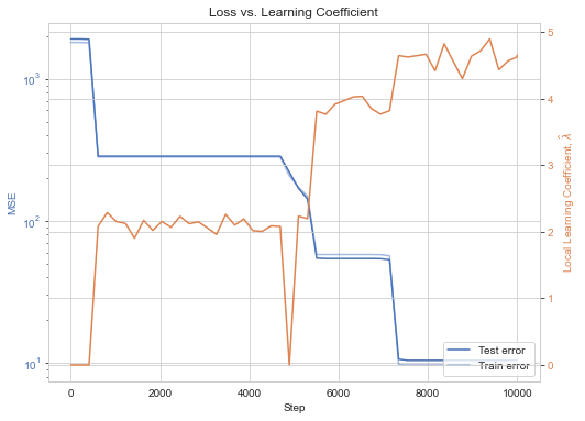
Deep linear networks. Let's consider the example of deep linear networks (DLNs). These are neural networks without nonlinear activations. In terms of expressivity, these models are identical to a simple affine transformation but in terms of dynamics they're much more interesting. The observed "saddle-to-saddle" transitions involve sudden jumps in the loss that coincide with sudden increases in the learning coefficient.
From Basins to Model Complexity
In this section, we'll motivate the learning coefficient by attempting to formalize a working definition of basin volume (through which we'll see that what we really care about is basin volume scaling). We'll see in what sense the learning coefficient measures model complexity and examine the resulting perspective on phase transitions.
Intractable: Basin Volume
Basin volume and model simplicity. Learning theorists have long been interested in the link between basin volume and model simplicity. We don't really care what model we end up with as long as its loss is below some threshold . This is particularly true as that threshold approaches its minimum: we want to know how many "almost-as-good" solutions there are in the neighborhood of an obtained solution .
Intuitively, broader basins (with more suitable models) are simpler. Because they take up more volume, they require fewer bits to locate. In accordance with Occam's razor, we want the simplest possible solution for the problem at hand.[1]
To measure a basin. In particular, given an upper bound to the loss , we want to compute the following volume (="area" in the case of two parameters):
for some prior over weights . For our purposes, we can safely neglect the prior and treat it as constant. Consider the toy loss landscape below, where is indicated by the gray projection.
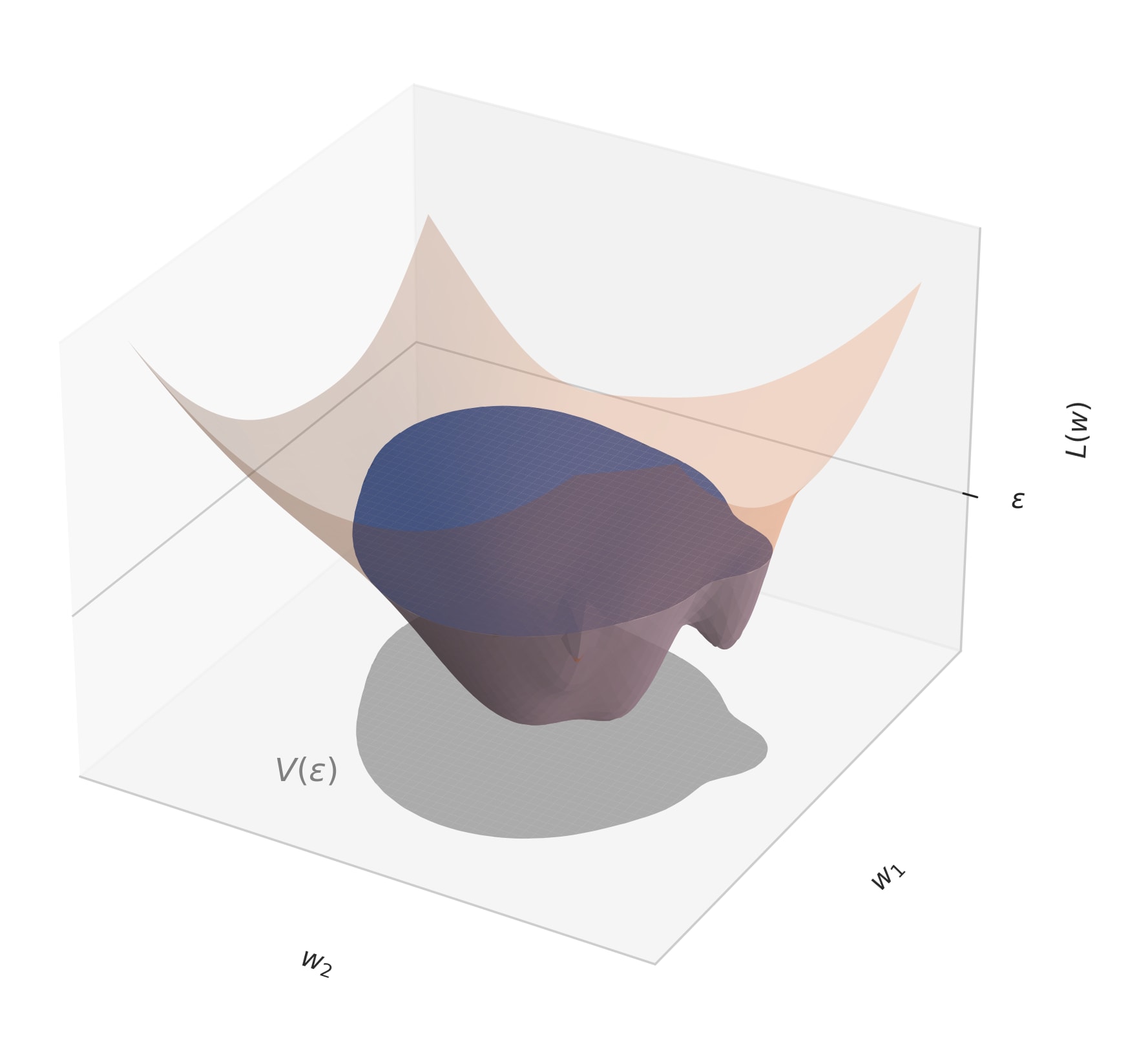
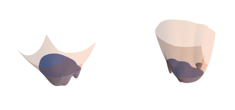
This is not a good representation of real-world loss landscapes.
Model complexity and comparison. Every model in a given basin has the same basin volume. This metric is a coarse-grained observable (much like volume in thermodynamics) that partitions weight space into subclasses of similar models. So seeing that two models have similar volumes increases the odds that they're computationally similar. Conversely, having different volumes / complexities suggests that two models are qualitatively distinct.
Unfortunately, actually computing basin volume is intractable. This is because of the curse of dimensionality (the volume scales exponentially with dimensions) and because we can only ever approximate the "true" population loss through an empirical loss evaluated on a finite dataset .
Wrong: Basin Flatness
From broadness to flatness. The usual workaround to this intractability is to use a Taylor expansion: as long as we're close enough to the bottom of the basin, we can approximate the basin locally with a polynomial.
Most people stop at a second-order approximation [LW · GW], modeling the basin as a paraboloid whose curvatures are given by the Hessian at the minimum. It's a simple matter of then computing the resulting surface volume.
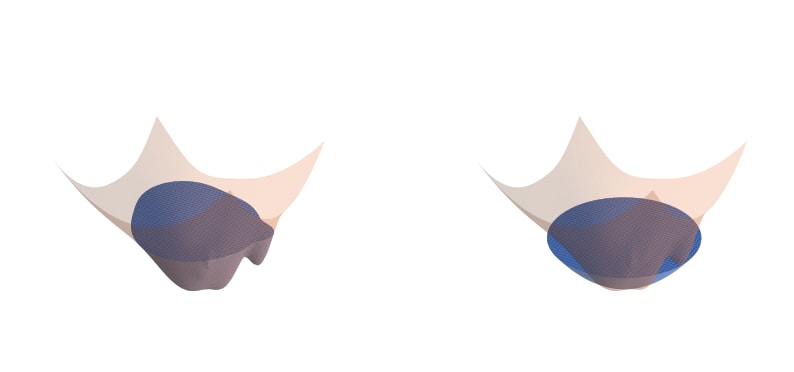
This is an invalid approximation.
Unfortunately, this approximation is wrong. Minimum flatness is a terrible proxy for basin volume. The fundamental problem is that neural networks are singular [LW · GW]: their loss landscapes have degenerate critical points. In practice, Hessians of the loss generally have many zero eigenvalues (often a majority). When we attempt to approximate the volume with a paraboloid that has zero curvature, we naively predict unphysical infinite volumes.
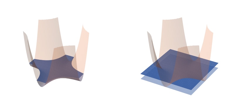
The standard correction is to add a small constant to these zero eigenvalues [LW(p) · GW(p)], which stabilizes the Hessian. We get a very large volume, instead of an infinite volume. But this misses the point: when second order terms vanish, the qualitative equivalence between a function and its second-order Taylor approximation breaks down, and these Hessian-based approximations become invalid.
Instead, we need to go to higher order terms in the Taylor expansion. The largest contributions to the volume will come from the first non-vanishing terms in the expansion.
Flatness ≠ broadness. In the literature, flatness (in the sense of a small determinant of the Hessian) and broadness often get conflated. This is unfortunate: the two are not the same. Basin broadness is an interesting question. Minimum flatness is the wrong question.
Instead: Basin Dimension
Volume dynamics. We care about relative — not absolute — volumes. But even more importantly, we're interested in dynamics: how the volume changes as learning progresses. As we gather more and more data, we're able to become more discriminating and our threshold comes down. The real question, then, is: how does the volume scale as changes? This is more relevant even in the non-degenerate regular case.
Volume scaling > volume. Studying volume scaling solves several others problems with the volume. First, for sufficiently small , relative volumes become independent of , which allows us to eliminate the dependence on this arbitrary cut-off. Furthermore, volume scaling is invariant under reparametrizations and non-diverging even near degenerate critical points.
The learning coefficient as effective dimensionality. The volume scales as
The scaling exponent is known as the learning coefficient (or "real log canonical threshold [LW · GW]"). It plays the role of an effective dimensionality (up to a constant multiple).
Let's illustrate this with some examples.
Regular models. First, consider the case of regular (=non-singular) models, where the loss landscape has no degenerate critical points. In this case, the Hessian-based approximation holds, and the volume grows with exponent , where is the number of dimensions (or parameter count).

Singular models. Consider the function . At the origin, the Hessian is equal to the zero matrix, and the learning coefficient is .

Compare this to the function . Again the Hessian at the origin is the zero matrix, but the learning coefficient now takes a different value .

For singular models, the parameter count sets an upper bound . Lower learning coefficient means the volume scales slower for for large but faster for small . There's exponentially more volume in the immediate vicinity of degenerate critical points than in the vicinity of non-degenerate critical points.
Against Hessians. The two preceding examples explicitly demonstrate the failures of the Hessian mentioned earlier. Their Hessians are identical at the origin, but their scaling behaviors are radically different. The Hessian is a poor judge of volume, and derived metrics like the rank of the Hessian are insufficient notions of model complexity.[2]
The learning coefficient as an inductive bias. The Occam's razor intuition that simpler models (with lower complexity) generalize better is formalized by Watanabe's free energy formula,
where is the number of training samples, is the loss (more precisely, the negative log likelihood) which depends on a dataset of samples, and is an optimal choice of weights.
A full explanation and derivation of this formula is beyond the scope of this post (see Liam's excellent sequence [LW · GW]), but the important bit is that we can construe the problem of Bayesian learning as a problem of trying to minimize this free energy, involving a tradeoff between accuracy (lower ) and complexity (lower ). Neural networks are intrinsically biased towards simpler solutions.
Intuition for phase transitions. Consider a toy landscape with two local minima at and with heights . Both minima have an associated learning coefficient that determines how the volume scales in its neighborhood. Suppose . Solution 1 is simpler but with higher loss, and solution 2 is more accurate but also more complex.
Coming back to the volume for a moment, what happens as we gradually lower the threshold ?

What we're interested in is the fraction of the surface area (=the volume of weight space) that is taken up by different kinds of solutions. At first, this surface area, and thus the behavior of our models, is dominated by the more degenerate solution at .
As we sample more data () the sea starts to recede. When the sea level approaches the level of one of these highly degenerate, low-accuracy solutions, that solution suddenly and very rapidly loses a massive amount of surface area precisely because it is so degenerate. Shallow puddles vanish all at once.
The fraction of surface area taken up by successive, more complex solutions jumps just as suddenly and rapidly. There's a phase transition — a qualitative change in the kind and complexity of functions being learned.
The sea continues to sink. From where we're sitting — above the water — we can't see below the surface. We don't know where or when the next transition will take place. We hold our breaths...
Estimating Learning Coefficients
We've seen what the learning coefficient is and how it measures the complexity of a model. But how can we go about practically estimating its value? In this section, we describe a set of techniques introduced by Lau et al. (2023).
Deriving the Estimator
From free energies to learning coefficients. The free energy formula we saw earlier,
offers a means of calculating the learning coefficient. We simply shuffle the terms around to obtain:
WBIC. Unfortunately, performing the integral required to evaluate is intractable. As an alternative, we can consider the Widely Applicable Bayesian Information Criterion (WBIC), which generalizes the Bayesian Information Criterion (BIC) to singular models,
where is the tempered Bayesian posterior,
sampled at inverse temperature (Watanabe, 2013). The two highest order terms in the expansion of the WBIC match that of the asymptotic expansion of , which means we can substitute this in for to estimate the learning coefficient:
Expectations to empirical averages. To use this estimator, we need to first estimate the expectation value . We can do this by sampling a set of weights and replacing the expectation value with an empirical average over the losses associated to those weights,
Unfortunately, estimating in practice runs into significant curse-of-dimensionality effects for systems at scale.
The Local Learning Coefficient
From global to local. The problem becomes substantially more tractable if, instead of attempting to estimate the global learning coefficient, we estimate a local learning coefficient instead. We restrict our attention to a subset of weights and study how the volume scales in just that region. The scaling is dominated by the most complex local singularities.
As we saw in the aside on phase transitions, this local quantity is also more interesting from the perspective of dynamics. When actually training models, we don't care about the behaviors of all possible models, we care about the behavior of a specific model as it moves through the loss landscape.

The local learning coefficient. To estimate the local learning coefficient, Lau et al. (2023) replace the prior with a localizing prior centered at the point whose learning coefficient we want to estimate:
This ensures that samples drawn will remain "close" to the original point. Substituting this into the global estimator we saw earlier, we obtain the definition of the local learning coefficient,
known colloquially as "lambda-hat," where indicates the use of a localizing prior.
To estimate this expectation value, we compute an empirical average over the losses of a set of samples , now drawn from the localized posterior:
Given this empirical average, we plug it into the above formula for (subtracting times the loss at and dividing by ) to obtain an estimate for the local learning coefficient.
Implementing the Estimator
How to localize? The first practical question we run into when implementing the local learning coefficient estimator is how to localize. Lau et al. consider a Gaussian prior parametrized by a scale . This is not the only possible choice, but it is perhaps the most straightforward choice: a gentle quadratic restoring force.
How to sample? To draw samples from the posterior , the natural thought is to use MCMC techniques. Explaining why these work is beyond the scope of this piece and is well covered elsewhere, but what's important here is that standard MCMC methods run into the curse of dimensionality, which makes them unsuitable for larger models.
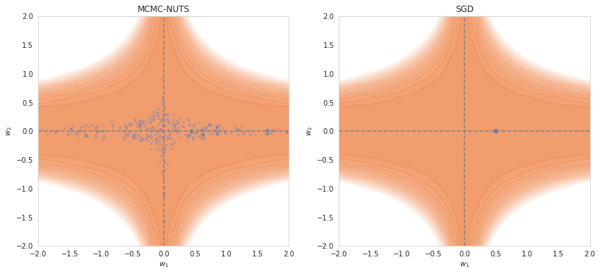
SGLD. To scale MCMC methods to higher dimensions, we need to incorporate information from gradients. This allows us to "preselect" low-loss, high-posterior regions of weight space. One of the simplest examples of such a technique is Stochastic Gradient Langevin Dynamics (SGLD), which is SGD with the addition of an explicit noise term (Welling & Teh 2011). This allows random movement along low loss dimensions, while quickly pushing any step to a higher loss area back down.
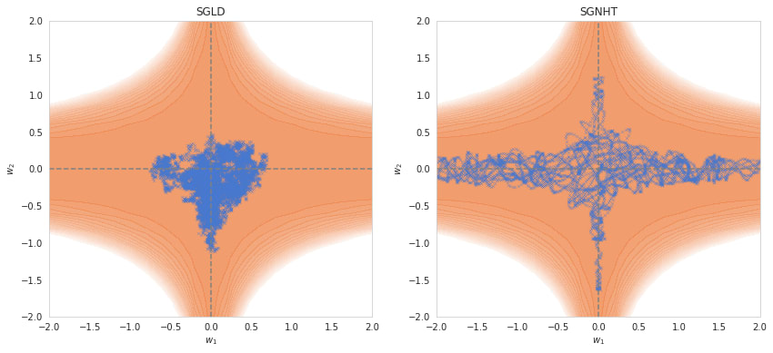
SGNHT and beyond. Adding momentum & friction would allow us to explore these ridges of the posterior more effectively. One such example is the Stochastic Gradient Nosé-Hoover Thermostat (SGNHT), which uses a thermostat for its friction term (Ding et al. 2014). Although clearly performing better in the toy potential above, it's still unclear how well this approach generalizes to higher dimensions as these samplers can be harder to get working than SGLD.
Limitations
Engineering limitations. The above estimators do not yet live up to their full theoretical potential. To give an example, depends on hyperparameters like the number of samples, the localizing strength , the SGLD learning rate , etc. The true coefficient is independent of these hyperparameters.
We care less about whether is an unbiased estimator of and more about whether this estimator satisfies certain basic desiderata of model complexity. These include properties like ordinality: that implies . Improving this estimator and confirming that it satisfies these desiderata is currently bottlenecked more on engineering than on theory.
Theoretical limitations. At the same time, this estimator sometimes exceeds its theoretical underpinnings, yielding sensible results despite violating certain technical assumptions. This means there's work to do for theorists in terms of finding assumptions to relax and studying, for example, how to extend the learning coefficient outside of non-minima. Currently, if not applied at a local minimum, the estimator can sometimes yield unphysical negative model complexities.[3]
There are limiting assumptions underlying the learning coefficient and additional limiting assumptions underlying the local learning coefficient. Both require further attention.
Proceed with caution. The current techniques for estimating are finicky to get working and should be applied with care. This is a research tool, not a plug-and-play observable printing press. Expect annoying hyperparameter tuning, (un)correlated estimates, weirdly high 's, negative 's, infinite 's, etc. This requires at least as much caution as MCMC in any other high-dimensional system: pay careful attention to diagnostics of chain health and vary hyperparameters to hunt for dependencies, systematic or otherwise.
What's Next
Improving estimates. An immediate priority is to confirm that and match where it counts. Does it satisfy our desiderata? And can we calibrate in settings where we can analytically derive ? There's work to do on the theoretical front and on the computational front in terms of exploring more scalable and more accurate ways to sample from the local posterior beyond SGLD.
More observables. SLT also tells us how to measure other quantities of interest, such as the singular fluctuation. We're also working on the second and third generations of techniques for studying transitions that extract vector and higher-order information about how models are changing.
Go forth and estimate! Although the current implementation is far from perfect, it should be good enough to start applying these techniques in practice. It's as easy as pip install devinterp and from devinterp.slt import estimate_learning_coeff (or at least, it's easy up until that point). We recommend checking out these example notebooks for inspiration.
If you want to learn more about the learning coefficient, see this post [LW · GW], this lecture, or this book. For updates on developmental interpretability, join the discord. Stay tuned for more updates soon!
Thank you to @Daniel Murfet [LW · GW], @Edmund Lau [LW · GW], @Alexander Gietelink Oldenziel [LW · GW], and @Liam Carroll [LW · GW] for reviewing early drafts of this document.
- ^
Actually extending the minimum description length principle ('choose the model that takes the fewest bits to specify') to singular models is an open problem. The free energy formula (covered later) is not quite the same, though it fulfills the same purpose of formalizing Occam's razor.
- ^
To give the Hessian some credit: its rank can give an us a lower bound on the model complexity. The Hessian still has its place. (EDIT: this originally said upper bound — that was wrong)
- ^
This occurs when the sampler strays beyond its intended confines and stumbles across models with much lower loss than those in the desired neighborhood.
17 comments
Comments sorted by top scores.
comment by TurnTrout · 2023-10-11T19:18:55.025Z · LW(p) · GW(p)
In particular, we're aiming to understand phase transitions during learning — moments in which models go through sudden, unanticipated shifts. We want to be able to detect these transitions because we think most of the risk is contained in sudden, undesired changes to values or capabilities that occur during training
Maybe a basic question, but why do you think dangerous capabilities will exhibit discrete phase transitions? My impression is that grokking indicates that generalizing subnetworks can be continuously upweighted over a training run, and I don't know at what point the subnetwork is "implemented" or not, as opposed to "more or less strongly weighted."
Replies from: jhoogland↑ comment by Jesse Hoogland (jhoogland) · 2023-10-12T00:20:54.584Z · LW(p) · GW(p)
We don’t necessarily expect all dangerous capabilities to exhibit phase transitions. The ones that do are more dangerous because we can’t anticipate them, so this just seems like the most important place to start.
It's an open question to what extent the lottery-ticket style story of a subnetwork being continually upweighted contradicts (or supports) the phase transition perspective. Just because a subnetwork's strength is growing constantly doesn't mean its effect on the overall computation is. Rather than grokking, which is a very specific kind of phase transition, it's probably better to have in mind the emergence of in-context learning in tandem with induction heads, which seems to us more like the typical case we're interested in when we speak about structure in neural networks developing across training.
We expect there to be a deeper relation between degeneracy and structure. As an intuition pump, think of a code base where you have two modules communicating across some API. Often, you can change the interface between these two modules without changing the information content being passed between them and without changing their internal structure. Degeneracy — the ways in which you can change your interfaces — tells you something about the structure of these circuits, the boundaries between them, and maybe more. We'll have more to say about this in the future.
↑ comment by gwern · 2023-11-05T17:01:03.811Z · LW(p) · GW(p)
it's probably better to have in mind the emergence of in-context learning in tandem with induction heads, which seems to us more like the typical case we're interested in when we speak about structure in neural networks developing across training.
The induction-bump seems like a good test case for the Bayesian basin interpretation.
One would really want to know if the complexity measure can predict 'emergence' of capabilities like inner-monologue, particularly if you can spot previously-unknown capabilities emerging which may not be covered in any of your existing benchmarks. But this type of 'emergence' tends to happen with such expensive models that the available checkpoints are too separated to be informative (if you get an emergence going from 1b vs 10b vs 100b, what does it mean to compute a complexity measure there? You'd really want to compare them at wherever the emergence actually really happens, like 73.5b vs 74b, or whatever.)
But the induction bump happens at pretty small (ie. cheap) model sizes, so it could be replicated many times and in many ways within-training-run and across training-runs, and one see how the complexity metric reflects or predicts the induction bump. Is that one of the 'hidden' transitions you plan to test? And if not, why not?
Replies from: jhoogland, jhoogland, kave↑ comment by Jesse Hoogland (jhoogland) · 2024-02-09T18:49:54.909Z · LW(p) · GW(p)
Our work on the induction bump is now out. We find several additional "hidden" transitions, including one that splits the induction bump in two: a first part where previous-token heads start forming, and a second part where the rest of the induction circuit finishes forming.
The first substage is a type-B transition (loss changing only slightly, complexity decreasing). The second substage is a more typical type-A transition (loss decreasing, complexity increasing). We're still unclear about how to understand this type-B transition structurally. How is the model simplifying? E.g., is there some link between attention heads composing and the basin broadening?
↑ comment by Jesse Hoogland (jhoogland) · 2023-11-16T09:15:05.747Z · LW(p) · GW(p)
One would really want to know if the complexity measure can predict 'emergence' of capabilities like inner-monologue, particularly if you can spot previously-unknown capabilities emerging which may not be covered in any of your existing benchmarks.
That's our hope as well. Early ongoing work on toy transformers trained to perform linear regression seems to bear out that lambdahat can reveal transitions where the loss can't.
But this type of 'emergence' tends to happen with such expensive models that the available checkpoints are too separated to be informative (if you get an emergence going from 1b vs 10b vs 100b, what does it mean to compute a complexity measure there? You'd really want to compare them at wherever the emergence actually really happens, like 73.5b vs 74b, or whatever.)
The kind of emergence we're currently most interested in is emergence over training time, which makes studying these transitions much more tractable (the main cost you're paying is storage for checkpoints, and storage is cheap). It's still a hurdle in that we have to start training large models ourselves (or setting up collaborations with other labs).
But the induction bump happens at pretty small (ie. cheap) model sizes, so it could be replicated many times and in many ways within-training-run and across training-runs, and one see how the complexity metric reflects or predicts the induction bump. Is that one of the 'hidden' transitions you plan to test? And if not, why not?
The induction bump is one of the main things we're looking into now.
↑ comment by kave · 2023-11-05T17:57:33.967Z · LW(p) · GW(p)
Looks like it's in-progress.
comment by Charlie Steiner · 2023-10-11T18:11:33.062Z · LW(p) · GW(p)
Pretty neat.
My ears perk up when I hear about approximations to basin size because it's related to the Bayesian NN model of uncertainty.
Suppose you have a classifier that predicts a probability distribution over outputs. Then when we want the uncertainty of the weights, we just use Bayes' rule, and because most of the terms don't matter we mostly carte that P(weights | dataset) has evidence ratio proportional to P(dataset | weights). If you're training on a predictive loss, your loss is basically the log of this P(dataset | weights), and so a linear weighting of probability turns into an exponential weighting of loss.
I.e. you end up (in theory that doesn't always work) with a Boltzmann distribution sitting at the bottom of your loss basin (skewed by a regularization term). Broader loss basins directly translate to more uncertainty over weights.
Hm... But I guess thinking about this really just highlights for me the problems with the approximations used to get uncertainties out of the Bayesian NN picture. Knowing the learning coefficient is of limited use because, especially when some dimensions are different, you can't really model all directions in weight-space as interchangeable and uncorrelated, so increased theoretical firepower doesn't translate to better uncertainty estimates as nicely as I'd like.
comment by Buck · 2023-11-05T21:16:32.643Z · LW(p) · GW(p)
(some of which we'd rather not expose our model to).
Why do you want to avoid exposing your model to some inputs?
Replies from: jhoogland↑ comment by Jesse Hoogland (jhoogland) · 2023-11-16T09:17:48.748Z · LW(p) · GW(p)
I think there's some chance of models executing treacherous turns in response to a particular input, and I'd rather not trigger those if the model hasn't been sufficiently sandboxed.
comment by Chris_Leong · 2023-10-12T10:39:16.638Z · LW(p) · GW(p)
Do phase transitions actually show up? So far, the places where theoretically predicted phase transitions are easiest to confirm are simplified settings like deep linear networks and toy models of superposition. For larger models, we expect phase transitions to be common but "hidden." Among our immediate priorities are testing just how common these transitions are and whether we can detect hidden transitions.
What do you mean by 'hidden"?
↑ comment by Daniel Murfet (dmurfet) · 2023-10-12T21:06:49.235Z · LW(p) · GW(p)
Not easily detected. As in, there might be a sudden (in SGD steps) change in the internal structure of the network over training that is not easily visible in the loss or other metrics that you would normally track. If you think of the loss as an average over performance on many thousands of subtasks, a change in internal structure (e.g. a circuit appearing in a phase transition) relevant to one task may not change the loss much.
comment by Vinayak Pathak (vinayak-pathak) · 2025-02-19T22:36:36.599Z · LW(p) · GW(p)
Neural networks are intrinsically biased towards simpler solutions.
Am I correct in thinking that being "intrinsically biased towards simpler solutions" isn't a property of neural networks, but a property of the Bayesian learning procedure? The math in the post doesn't use much about NN's and it seems like the same conclusions can be drawn for any model class whose loss landscape has many minima with varying complexities?
Replies from: jhoogland↑ comment by Jesse Hoogland (jhoogland) · 2025-02-19T23:45:56.902Z · LW(p) · GW(p)
To be precise, it is a property of singular models (which includes neural networks) in the Bayesian setting. There are good empirical reasons to expect the same to be true for neural networks trained with SGD (across a wide range of different models, we observe the LLC progressively increase from ~0 over the course of training).
comment by Michael Pearce (michael-pearce) · 2023-11-16T01:42:16.921Z · LW(p) · GW(p)
The characterization of basin dimension here is super interesting. But it sounds like most of the framing is in terms of local minima. My understanding is that saddle points are much more likely in high dimensional landscapes (eg, see https://arxiv.org/abs/1406.2572) since there is likely always some direction leading to smaller loss.
How does your model complexity measure work for saddle points? The quotes below suggest there could be issues, although I imagine the measure makes sense as long as the weights are sampled around the saddle (and not falling into another basin).
Currently, if not applied at a local minimum, the estimator can sometimes yield unphysical negative model complexities.
Replies from: dmurfetThis occurs when the sampler strays beyond its intended confines and stumbles across models with much lower loss than those in the desired neighborhood.
↑ comment by Daniel Murfet (dmurfet) · 2024-01-11T03:29:16.519Z · LW(p) · GW(p)
This is an open question. In practice it seems to work fine even at strict saddles (i.e. things where there are no negative eigenvalues in the Hessian but there are still negative directions, i.e. they show up at higher than second order in the Taylor series), in the sense that you can get sensible estimates and they indicate something about the way structure is developing, but the theory hasn't caught up yet.