[PAPER] Jacobian Sparse Autoencoders: Sparsify Computations, Not Just Activations
post by Lucy Farnik (lucy.fa) · 2025-02-26T12:50:04.204Z · LW · GW · 8 commentsContents
  Summary of the paper
    TLDR
    Why we care about computational sparsity
    Jacobians ≈ computational sparsity
    Core results
  How this fits into a broader mech interp landscape
    JSAEs as hypothesis testing
    JSAEs as a (necessary?) step towards solving interp
  Call for collaborators
  In-the-weeds tips for training JSAEs
None
8 comments
We just published a paper aimed at discovering “computational sparsity”, rather than just sparsity in the representations. In it, we propose a new architecture, Jacobian sparse autoencoders (JSAEs), which induces sparsity in both computations and representations. CLICK HERE TO READ THE FULL PAPER.
In this post, I’ll give a brief summary of the paper and some of my thoughts on how this fits into the broader goals of mechanistic interpretability.
Summary of the paper
TLDR
We want the computational graph corresponding to LLMs to be sparse (i.e. have a relatively small number of edges). We developed a method for doing this at scale. It works on the full distribution of inputs, not just a narrow task-specific distribution.
Why we care about computational sparsity
It’s pretty common to think of LLMs in terms of computational graphs. In order to make this computational graph interpretable, we broadly want two things: we want each node to be interpretable and monosemantic, and we want there to be relatively few edges connecting the nodes.
To illustrate why this matters, think of each node as corresponding to a little, simple Python function, which outputs a single monosemantic variable. If you have a Python function which takes tens of thousands of arguments (and actually uses all of them to compute its output), you’re probably gonna have a bad time trying to figure out what on Earth it’s doing. Meanwhile, if your Python function takes 5 arguments, understanding it will be much easier. This is what we mean by computational sparsity.
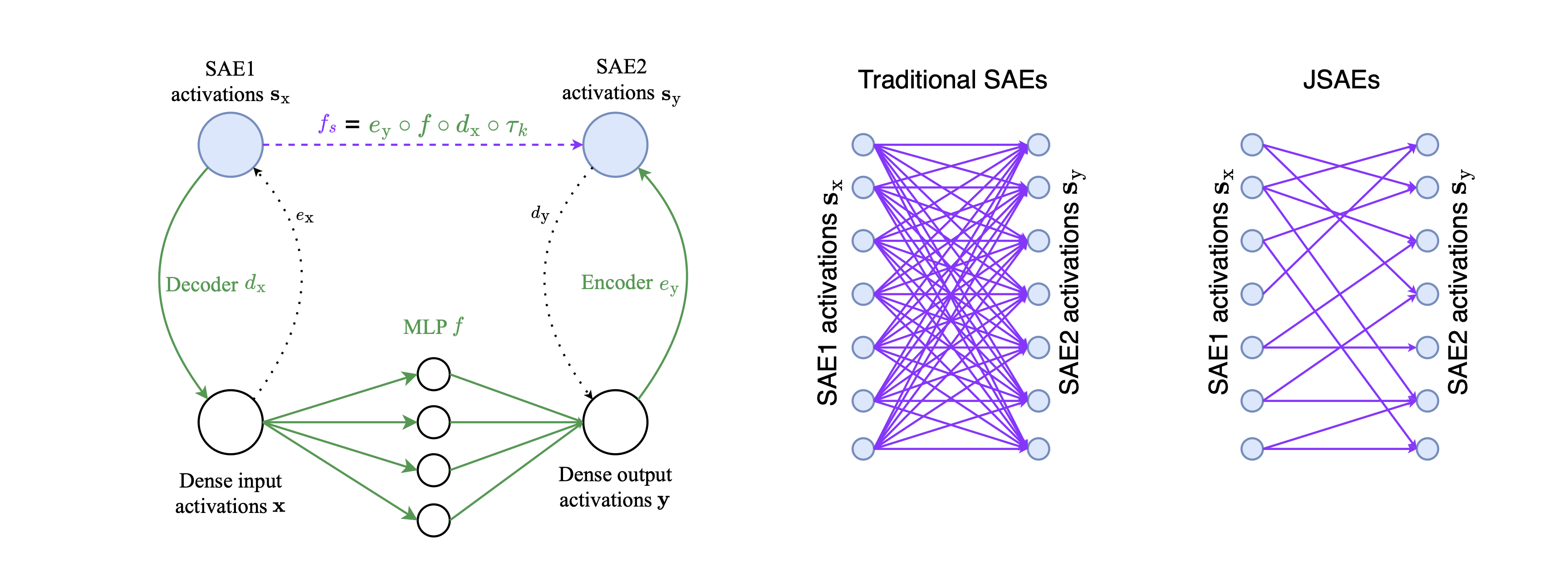
More specifically in our paper, we “sparsify” the computation performed by the MLP layers in LLMs. We do this by training a pair of SAEs — the first SAE is trained on the MLP’s inputs, the second SAE is trained on the MLP’s outputs. We then treat the SAE features as the nodes in our computational graph, and we want there to be as few edges connecting them as possible without damaging reconstruction quality.
Jacobians computational sparsity
We approximate computational sparsity as the sparsity of the Jacobian. This approximation, like all approximations, is imperfect, but it is highly accurate in our case due to the fact that the function we are sparsifying is approximately linear (see the paper for details).
Importantly, we can actually compute the Jacobian at scale. This required some thinking, since naively the Jacobian would be of size , which would have trillions of elements even for very small LLMs and would result in OOM errors. But we came up with a few tricks to do this really efficiently (again, see the paper for details). With our set up, training a pair of JSAEs takes only about twice as long as training a single standard SAE.
We compute the Jacobians at each training step and add an L1 sparsity penalty on the flattened Jacobian to our loss function.
Core results
- The Jacobians when using JSAEs are indeed much more sparse than the Jacobians when using a pair of traditional SAEs.
- JSAEs achieve this without damaging reconstruction quality. There’s only a small trade-off between Jacobian sparsity and reconstruction quality. (Note that sparsity of the SAE activations is fixed since we’re using TopK SAEs.)
- JSAEs also get the same auto-interp scores. In fact they may somewhat outperform traditional SAEs on this, but that may not be statistically significant. Note that we’re using fuzzing for this which may be problematic in some circumstances (see our previous paper).
- The Jacobians are much more sparse in pre-trained LLMs than in re-initialized transformers. This indicates that computational sparsity emerges during training, which means JSAEs are likely picking up on something “real”, at least in some sense. (Of course there are caveats to that last sentence, I won’t get into them here.).
- The function we are “sparsifying”, corresponding to the MLP when re-written in the basis found by JSAEs, is almost entirely linear. This is important because, for a linear function, the Jacobian perfectly measures causal relations — a partial derivative of zero in a linear function implies there is no causal connection.
How this fits into a broader mech interp landscape
(Epistemic status of this section: speculations backed by intuitions, empirical evidence for some of them is limited/nonexistent)
JSAEs as hypothesis testing
If we ever want to properly understand what LLMs are doing under the hood, I claim that we need to find a “lens” of looking at them which induces computational sparsity.
Here is my reasoning behind this claim. It relates to a fuzzy intuition about “meaning” and “understanding”, but it’s hopefully not too controversial: in order to be able to understand something, it needs to be decomposable. You need to be able to break it down into small chunks. You might need to understand how each chunk relates to a few other parts of the system. But if, in order to understand each chunk, you need to understand how it relates to 100,000 other chunks and you cannot understand it in any other way, you’re probably doomed and you won’t be able to understand it.
“Just automate mech interp research with GPT-6” doesn’t solve this. If there doesn’t exist any lens in which the connections between the different parts are sparse, what would GPT-6 give you? It would only be able to give you an explanation (whether in natural language, computer code, or equations) that has these very dense semantic connections between different concepts, and my intuition is that this would be effectively impossible to understand (at least for humans anyway). Again, imagine a python function with 10,000 arguments, all of which are used in the computation, which cannot be rewritten in a simpler form.
Either we can find sparsity in the semantic graph, or interpretability is almost certainly doomed. This means that one interpretation of our paper is testing a hypothesis. If computational sparsity is necessary (though not sufficient) for mech interp to succeed, and without computational sparsity mech interp would be doomed, is there computational sparsity? We find that there is, at least in MLPs.
JSAEs as a (necessary?) step towards solving interp
In order to solve interpretability, we need to solve a couple of sub-problems. One of them is disentangling activations into monosemantic representations, which are hopefully human-interpretable. Another one is finding a lens using those monosemantic representations which has sparsity in the graph relating these representations to one another. SAEs aim to solve the former, JSAEs aim to solve the latter.
On a conceptual level, JSAEs take a black box (the MLP layer) and break it down into tons of tiny black boxes. Each tiny black box takes as input a small handful of input features (which are mostly monosemantic) and returns a single output feature (which is likely also monosemantic).
Of course, JSAEs are almost certainly not perfect for this. Just like SAEs, they aim to approximate a fundamentally messy thing by using sparsity as a proxy for meaningfulness. JSAEs likely share many of the open problems of SAEs (e.g. finding the complete set of learned representations, including the ones not represented in the dataset used to train the SAE, which is especially important for addressing deceptive alignment). In addition to that, they probably add other axes along which things can get messy — maybe the computational graphs found by JSAEs miss some important causal connections, because the sparsity penalty probably doesn’t perfectly incentivize what we actually care about. That is one space for exciting follow-up work: what do good evals for JSAEs look like? How do you determine if the sparse causal graph JSAEs find is “the true computational graph”, what proxy metrics could we use here?
Call for collaborators
If you’re excited about JSAEs and want to do some follow-up work on this, I’d love to hear from you! Right now, as far as I’m aware, I’m the only person doing hands-on work in this space full-time. JSAEs (and ‘computational sparsity discovery’ in general) are severely talent-constrained. There are tons of things I would’ve loved to do in this paper if there had been more engineering-hours.
If you’re new to AI safety, I’d be excited to mentor you if we have personal fit! If you’re a bit more experienced, we could collaborate, or you could just bounce follow-up paper ideas off of me. Either way, feel free to drop me an email or DM me on Twitter.
Relatedly, I have a bunch of ideas for follow-up projects on computational sparsity that I’d be excited about. If you’d like to increase the probability of me writing up a “Concrete open problems in computational sparsity” LessWrong post, let me know in the comments that you’re interested in seeing this.
In-the-weeds tips for training JSAEs
If you’re just reading this post to get a feel for what JSAEs are and what they mean for mech interp, I’d recommend skipping this section.
- For the Jacobian sparsity loss coefficient (lambda in the paper), a good starting point is probably . Partially based on intuitions and partially based on limited empirical evidence, I speculate that this will often be the sweet spot.
- Do not use autodiff or anything similar for computing the Jacobians. We have an efficient method for doing this which only involves 3 mat muls, see the paper/code. Our current code for this works for GPT-2-style MLPs, if you’re using it on GLUs you’ll need to tweak the formulas (which shouldn’t be too hard) — you’re welcome to submit a PR for that.
- There are other ways to encourage sparsity besides the L1 penalty. We experimented with about a dozen (the code is included on our GitHub), and quite liked SCAD which seems to be a slight Pareto improvement over L1. We ultimately just went with the L1 in the paper for the sake of simplicity, but you might want to try SCAD for your use case. If you’re using our code base, just specify
-s scadwhen using thetrain.pyrunner. - You could use any activation function, but TopK makes things easier. Your “sliced” Jacobian (containing all the non-zero elements) for each token will be of size . If these vary between different tokens, you’ll have a harder time storing the Jacobians for your batch. Specifically you’ll need to implement masking and then you’ll need to decide how to appropriately “distribute the optimization pressure” between the different token positions. This is all very doable, but with TopK the size of your Jacobian is fixed at , so you don’t need to worry about these things.
- Measuring how sparse your Jacobians are is kind of tricky. Since there is no mechanism for producing exact zeros, L0 doesn’t work at all. Instead, the intuitive metric to use is a modified version of L0 where you measure the number of elements with absolute values above a small threshold (and discard the rest as “effectively 0”). However, this metric can get confounded by the fact that the L1 penalty encourages your Jacobians to get smaller. One way to mitigate this is to first normalize your Jacobians by a norm which heavily indexes on tail-end elements (e.g. or ), then measure the number of elements with absolute values above small thresholds, but that comes with its own problems. I’m mostly leaving the question of how to evaluate this properly to future work.
8 comments
Comments sorted by top scores.
comment by jacob_drori (jacobcd52) · 2025-02-26T22:03:09.001Z · LW(p) · GW(p)
The Jacobians are much more sparse in pre-trained LLMs than in re-initialized transformers.
This would be very cool if true, but I think further experiments are needed to support it.
Imagine a dumb scenario where during training, all that happens to the MLP is that it "gets smaller", so that MLP_trained(x) = c * MLP_init(x) for some small c. Then all the elements of the Jacobian also get smaller by a factor of c, and your current analysis -- checking the number of elements above a threshold -- would conclude that the Jacobian had gotten sparser. This feels wrong: merely rescaling a function shouldn't affect the sparsity of the computation it implements.
To avoid this issue, you could report a scale-invariant quantity like the kurtosis of the Jacobian's elements divided by their variance-squared, or ratio of L1 and L2 norms, or plenty of other options. But these quantities still aren't perfect, since they aren't invariant under linear transformations of the model's activations:
E.g. suppose an mlp_out feature F depends linearly on some mlp_in feature G, which is roughly orthogonal to F. If we stretch all model activations along the F direction, and retrain our SAEs, then the new mlp_out SAE will contain (in an ideal world) a feature F' which is the same as F but with larger activations by some factor. On the other hand, the mlp_in SAE should will contain a feature G' which is roughly the same as G. Hence the (F, G) element of the Jacobian has been made bigger, simply by applying a linear transformation to the model's activations. Generally this will affect our sparsity measure, which feels wrong: merely applying a linear map to all model activations shouldn't change the sparsity of the computation being done on those activations. In other words, our sparsity measure shouldn't depend on a choice of basis for the residual stream.
I'll try to think of a principled measure of the sparsity of the Jacobian. In the meantime, I think it would still be interesting to see a scale-invariant quantity reported, as suggested above.
Replies from: lucy.fa↑ comment by Lucy Farnik (lucy.fa) · 2025-02-27T18:00:52.378Z · LW(p) · GW(p)
I agree with a lot of this, we discuss the trickiness of measuring this properly in the paper (Appendix E.1) and I touched on it a bit in this post (the last bullet point in the last section). We did consider normalizing by the L2, ultimately we decided against that because the L2 indexes too heavily on the size of the majority of elements rather than indexing on the size of the largest elements, so it's not really what we want. Fwiw I think normalizing by the L4 or the L_inf is more promising.
I agree it would be good for us to report more data on the pre-trained vs randomized thing specifically. I don't really see that as a central claim of the paper so I didn't prioritize putting a bunch of stuff for it in the appendices, but I might do a revision with more stats on that, and I really appreciate the suggestions.
comment by leogao · 2025-02-27T19:36:05.424Z · LW(p) · GW(p)
Overall very excited about more work on circuit sparsity, and this is an interesting approach. I think this paper would be much more compelling if there was a clear win on some interp metric, or some compelling qualitative example, or both.
Replies from: lucy.fa↑ comment by Lucy Farnik (lucy.fa) · 2025-02-27T20:47:21.285Z · LW(p) · GW(p)
Completely agree! As I said in the post
> There are tons of things I would’ve loved to do in this paper if there had been more engineering-hours.
comment by Jacob Dunefsky (jacob-dunefsky) · 2025-02-27T19:09:12.724Z · LW(p) · GW(p)
This is very cool work!
One question that I have is whether JSAEs still work as well on models trained with gated MLP activation functions (e.g. ReGLU, SwiGLU). I ask this because there is evidence suggesting that transcoders don't work as well on such models (see App. B of the Gemmascope paper; I also have some unpublished results that I'm planning to write up that further corroborate this). It thus might be the case that the same greater representational capacity of gated activation functions causes both transcoders and JSAEs to be unable to learn sparse input-output mappings. (If both JSAEs and transcoders perform worse on gated activation functions, then I think that would indicate that there's something "weird" about these activation functions that should be studied further.)
comment by TheManxLoiner · 2025-02-27T15:14:05.327Z · LW(p) · GW(p)
If you’d like to increase the probability of me writing up a “Concrete open problems in computational sparsity” LessWrong post
I'd like this!
comment by Nikita Balagansky (nikita-balaganskii) · 2025-02-27T06:05:35.250Z · LW(p) · GW(p)
While authors claim that their approach is fundamentally different from transcoders [LW · GW], from my perspective, it addresses the same issue: finding interpretable circuits. I agree that it modulates MLPs in different ways (e.g., connecting sparse inputs and sparse outputs, rather than modulating MLP directly). However, it would be great to see the difference between circuits identified by transcoders and those found by JSAE.
We also discuss this similarity in Appendix F of our recent work (where transition T is analogous to f ), though we do not consider gradient-based approaches. Nevertheless, the most similar features between input and output can still sufficiently explain feature dynamics being a good baseline.
comment by joseph_c (cooljoseph1) · 2025-03-02T07:54:14.406Z · LW(p) · GW(p)
I'm a little confused about which computation you're trying to sparsify. The paper seems to be written in the context of the technique where one uses sparse autoencoders to extract "features" from the embedding space of large language models which are hopefully interpretable. (Please correct me if I'm wrong about that!)
The goal would seem to be, then, to sparsify the computation of the language model. However, the method in your paper seems to sparsify the computation of the autoencoders themselves, not the language model. Shouldn't the goal be to sparsify the language model's computation? If so, why not use weight pruning? What is JSAE better at?