Great-Filter Hard-Step Math, Explained Intuitively
post by Daniel_Eth · 2021-11-01T23:45:52.634Z · LW · GW · 7 commentsContents
  Introduction
  A simple model – “Try-Once” and “Try-Try” Steps
  A sequence of one try-try step
  A sequence of two try-try steps
  A sequence with n try-try steps
  A couple points of clarification
  Limitations of this model, and implications of expansions
None
7 comments
Crossposted to the EA Forum [EA · GW].
Introduction
The idea of the great filter was developed by Robin Hanson in 1998, building on some earlier work by Brandon Carter from 1983. The basic idea is that, since we see a lot of dead matter in the universe, and no good evidence of any technologically advanced, intergalactic civilizations expanding at a substantial fraction of the speed of light, then any proposed pathway by which the former might spontaneously develop into the latter must only ever happen with extremely small probability (given the size of the observable universe, most likely <<10^-20 per planetary system over several billion years).
We can, however, craft a sequence of steps whereby this extremely unlikely process could occur. Such a sequence of steps could include:
- Formation of a habitable celestial body (eg., contains liquid water, organics, etc)
- Formation or arrival of complex biomolecules
- Simple cells (eg., prokaryotes)
- Complex cells (eg., eukaryotes)
- Efficient meta-improvement to evolutionary algorithm (eg., sexual reproduction)
- Multicellularity
- Development of cells for efficient information processing (eg., neurons)
- Diversification and increased complexity of both the parts for and types of multicellular life (eg., during the Cambrian explosion)
- Evolution of a lifeform capable of higher-level reasoning, communication via language, building collective, intergenerational knowledge via cooperation and cumulative culture, and manipulating the physical world via fine-motor control (eg., humans)
- Development of mathematics, science, and engineering
- Development of advanced, spacefaring technology
- Explosive space colonization
Assuming this sequence as a whole is extremely unlikely, at least one of these steps must be very unlikely conditional on having passed all previous steps (ie., it must be a “hard step”), though it’s also possible that some of the steps are “easy steps”, passed with high probability (conditional on having passed the previous steps).
A simple model – “Try-Once” and “Try-Try” Steps
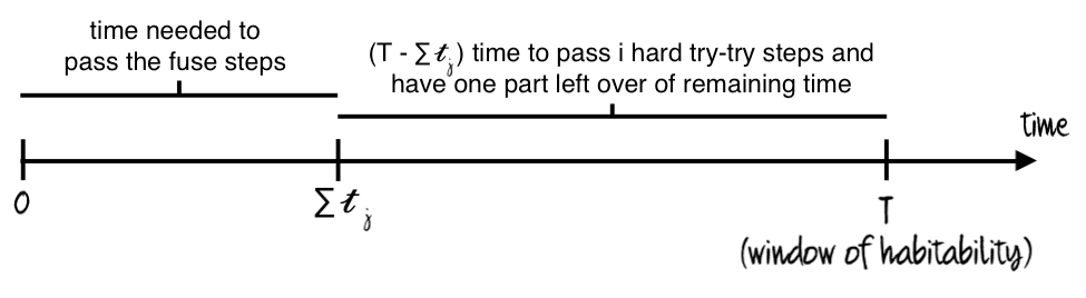
A simple model of this sequence could break down the steps into “try-once” steps (in which there is one chance to pass the step, and failure to pass it is permanent) and “try-try” steps (in which the step can be continuously attempted) which must all be passed in series within a time window equal to the habitability of the celestial body.
From the above sequence, step 1 (habitable celestial body) is probably best modeled as a try-once step, while the other steps are arguably better modeled as try-try steps (eg., step 3 – random complex biomolecules bumping into each other in the right way to happen to form simple cells – doesn’t necessarily become harder due to not having bumped together in the right way yet).
If we focus on the portion of these steps that have already been passed on Earth since its formation/habitabilization, then we are arguably left with a series of nine try-try steps (steps 2-10), which were passed over a period of 4.5 billion years, and with likely ~1 billion years remaining until Earth stops being habitable to complex, multicellular life (implying a total window of ~5.5 billion years).
A further simplification to the model could say that the chance of passing each try-try step doesn’t change over time (assuming that the step hasn’t already been passed, and that the previous step has been passed); we could call the corresponding probability of passing step i, within any one moment that it’s attempted, Ci (ie., this is equivalent to rolling an n-sided die until the number 1 is rolled, with Ci ~ 1/n).
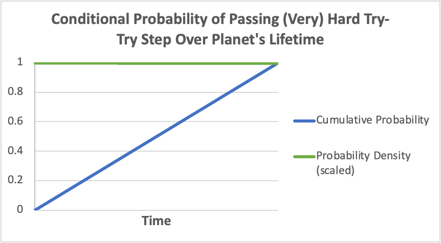
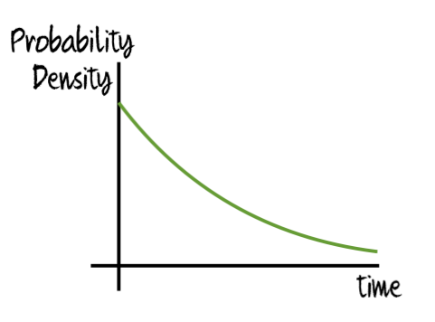
If we wanted to calculate the resultant probability of the step being passed at any one point in time (ie., the “probability density” of the step being passed at that time), starting with when the step is first attempted, we would need to multiply Ci by the probability that the step had not already been passed. As the cumulative probability of the step having already been passed must increase with time, the probability density of the step being passed must decrease with time (ie., the chance we’d have already rolled a 1 on the die would have increased, in which case we’d have already stopped rolling), as in the following graph (note that probability density here is scaled to be easily viewable on the same chart as the cumulative probability):
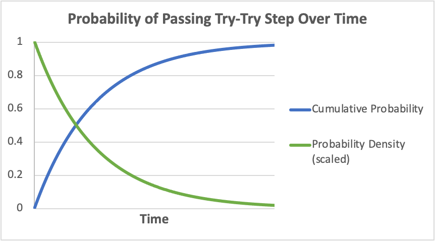
Mathematically, the probability density here can be described by what’s known as “exponential decay”, with the function: P ~ e^(-λt), where λ is the “rate constant” (related to Ci, above) and t is time. According to this function, the expected time to complete the step, 𝜏, is given by: 𝜏 = 1/λ (in the n-sided die example 𝜏 ~ n, meaning the more sides of the die, the longer expected time to roll a 1).
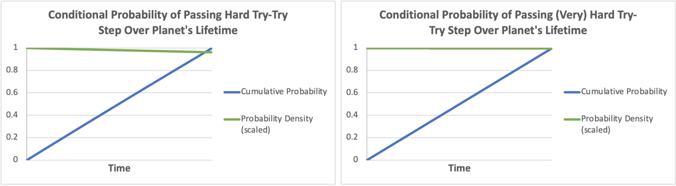
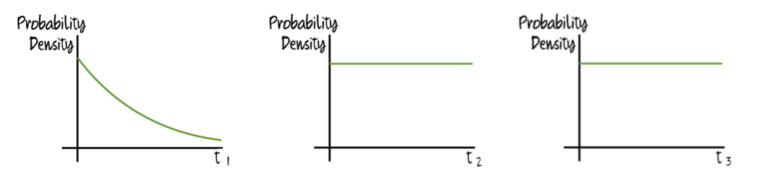
The various values of 𝜏 for the different try-try steps can vary by many orders of magnitude from each other, and also from the habitability window of the celestial body, T. As the value of T is set, largely, by geological, astronomical, and climatic factors (affecting things such as the existence of liquid water on the planet), while the values for the various 𝜏 would instead be set, primarily, by macroevolutionary factors employing completely different mechanisms (such as the rate of speciations and the likelihood of various biochemical reactions), it would be awfully coincidental if any specific 𝜏i had value 𝜏i ≈ T. Instead, we would a priori expect that for any given step, 𝜏i << T (implying step i is an easy step) or 𝜏i >> T (implying step i is a hard step).
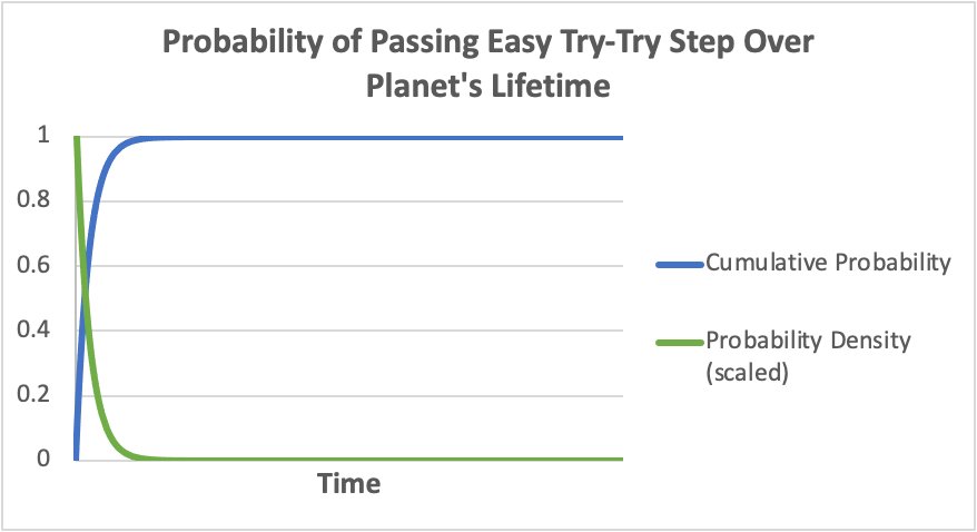
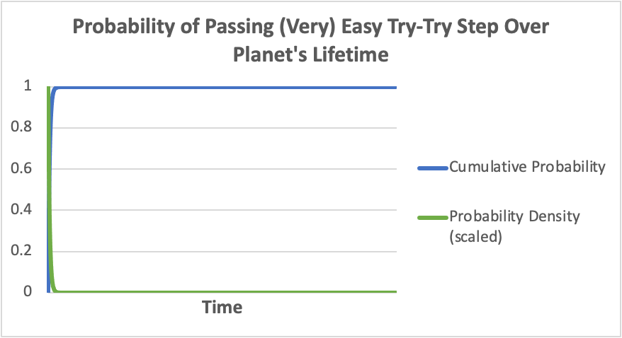
If 𝜏i << T, then the chance of passing the step over a time period equal to the planet’s lifetime (0 ≤ t ≤ T) would be something like this:
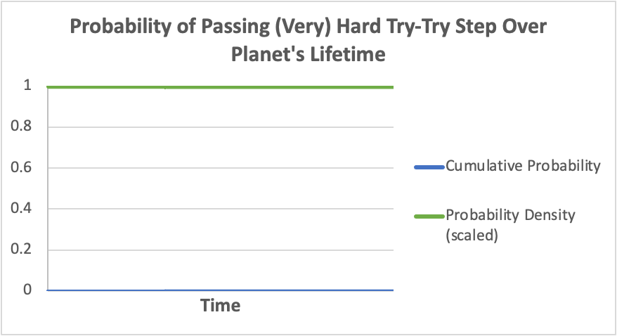
while if 𝜏i >> T, the chance of passing the step over a time period equal to the planet’s lifetime (0 ≤ t ≤ T) would be something like this:

The second of these still has the same basic formula (P ~ e^(-λt)), and is achieved by simply “zooming in” on the early part of a very long/wide graph of exponential decay.
One point of clarification – while T is an upper bound on how long any step can take to complete in the real world, there is no reason that 𝜏i cannot be larger than this, as 𝜏i is an abstract concept based on the value of λ and corresponds to how long the step would be expected to take in the hypothetical situation in which it was given an arbitrarily long time to complete and the habitability window was indefinitely long. Similarly, the above graphs give the entire window of T to the step in question; physically, this would only make sense if we were considering the first step, but mathematically, there’s no reason we can’t ask about any other steps, “How likely would this particular step be passed over a time period T, if the planet stayed habitable long enough for this particular step to be attempted for a time period T?” in which case the above graphs are appropriate.
Given the assumptions in the try-try model described here, a couple of statistical results are derivable that many people find intuitively surprising. First, if a sequence of steps on some planet has already been passed AND that sequence contains multiple hard try-try steps, then the expected time to complete each of these hard try-try steps would be almost exactly the same, even if some of these hard steps were MUCH harder than others of them. Second, if a sequence of steps on some planet has already been passed AND that sequence contains at least one hard try-try step, then the expected time remaining in the window of habitability of the planet since the last step was passed is ALSO almost exactly equal to the expected time of passing one of the hard try-try step(s).
The first of the above points implies that, for hard try-try steps, we cannot infer from the fossil record the relative difficulty of these steps based on the relative time it took to complete them. The second of the above points implies that the hard try-try step time on Earth may be ~1 billion years, the expected time until Earth will stop being habitable to large, complex life (though this value has large uncertainty and could be as large as several billion years or as small as a few hundred million years).
However, confusion over the reasoning behind these results leads to misunderstandings about their applicability, as well as what implications we’d expect if we change the model somewhat (for instance, by introducing the continual possibility of Earth losing habitability due to a freak astronomical or climatic event). In the remainder of this piece, I explain the reasoning behind these results as intuitively as I can, before concluding with potential expansions on the model and their implications.
Let’s start with examining a sequence of just a single try-try step.
A sequence of one try-try step
In this situation, there is one step, which takes time t1 to pass, and the step is passed iff this time is less than the planet’s window of habitability, T.
If the step is an easy step, then the probability distribution for t1, restricted to a domain equal to T (ie., over the planet’s habitability window), will familiarly look like the graph above for easy steps (reproduced below):
A few things stand out from this graph. First, it is overwhelmingly likely that the step will be passed in time (ie., with very high probability, t1 < T). Second, the expected value of t1 is given by E(t1) ≈ 𝜏1 = 1/λ1 << T/2.
It should be clear from the above that the easier we make the step, the smaller t1 will be in expectation:
Note that if the rate of passing the step, λ1, increases by a factor of 10, then the expected time to complete the step, E(t1), reduces by a factor of 10.
If the step is a hard step, however, then we get something qualitatively different for the probability distribution for t1(again, restricted to a domain equal to T). Again, the probability distribution will look like that above for hard steps (reproduced below):
In effect, the cumulative probability of passing the step (blue line) remains so low within this time window, that the probability density (green line) hardly declines over this time. If we condition on the step being passed in time (that is, the rare cases where t1 ≤ T), then we get this:

The relevant features are that the probability density (green) is approximately the uniform distribution, while the cumulative probability (blue) is approximately linear.
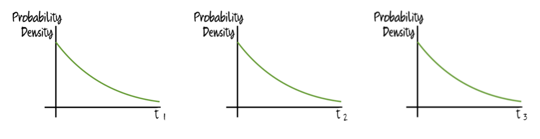
The expected time to pass the step, conditional on passing it within the window, is given by: E(t1 | t1 ≤ T) ≈ T/2 (due to ~symmetry, and the fact that the probability density is almost unchanged within this interval). Of course, this also means that the expected time remaining after passing the step, conditional on passing it, is: E(T - t1 | t1 ≤ T) ≈ T/2. Crucially, these results hold regardless of how hard the step is, assuming that it is, in fact, a hard step. The above graphs are made with a step that is assumed to be passed within T with a cumulative probability of ~4%, but if we instead assumed the chances of passing the step within this interval were only ~1/1M, we still get very similar results, with the following all-things-considered probabilities for t1:
and the following probabilities for t1, conditional on t1 ≤ T:
Again, E(t1 | t1 ≤ T) ≈ T/2. The harder hard step is likely to screen out many more worlds than the easier hard step, but conditional on not screening out a world, it isn’t expected to take any longer, since the probability distributions they present (in the relevant time window, conditional on passage) are almost identical.
Now, let’s move on to a situation with two try-try steps.
A sequence of two try-try steps
In this situation, we have two steps, s1 and s2, which take t1 and t2 to pass, respectively, and which must be completed in series before the planet’s habitability window closes (ie., within a time of T) for the sequence to be completed (that is, the sequence is completed iff t1 + t2 ≤ T).
If both of the steps are easy steps, then the situation is pretty straightforward: E(t1) = 𝜏1 << T/2, and E(t2) = 𝜏2 << T/2, so E(t1 + t2) = 𝜏1 + 𝜏2 << T, and the sequence is very likely to be completed. The easier of the two steps will also tend to be completed faster than the other (or course, the first of these steps will be completed earlier, but that's a different question).
If one of the steps is easy and the other step is hard, then the situation is still pretty simple. Let’s assume that s1 is the easy step and s2 is the hard step (it doesn’t actually matter which of the steps is which, since all that matters for passing the sequence is if t1 + t2 ≤ T, and this condition isn’t affected by the order of steps being switched; ie., t1 + t2 = t2 + t1). The first step will generally be passed quickly, as this is an easy step. Assuming the first step is passed, the remaining time (T - t1) is left for the second step. Note that this is similar to having a sequence of one hard try-try step (as in the above section), except the window for completing the step is no longer the entire habitable window of the planet, T, but instead the portion of that window that the first step didn’t eat into (T - t1).
Using similar reasoning to in the previous section, we would still expect the probability density of passing s2 to hardly change over time (from the moment s1 is passed until the planet stops being habitable) since the cumulative probability of passing s2 will remain small during the window we’re concerned with. Therefore, if we condition on s2 being passed, the probability density of passing this step (from the moment s2 is first attempted at time t1 until the planet stops being habitable at time T) will again approximate a uniform distribution. The expected value for t2 conditioning on passing the sequence will again be half of the window that s2 had (in this case that gives (T - t1)/2), and the expected remaining time after both steps are passed, conditional on both being passed, will therefore also be (T - t1)/2.
The situation becomes a bit more complicated if both steps are hard steps. In that case, s1 is probably not completed in time (that is, most likely, t1 > T). However, if s1 is completed in time (ie., t1 < T), then there is (T - t1) time left for s2. As with the situation in the above paragraph, the probability density of passing s2 does not appreciably decline over this window. Therefore, conditional on s2 being passed, the expected time that it took to pass would be almost exactly halfway through this window, with the other half of the window remaining – that is, the expected value of t2 conditional on passing the sequence would be (T - t1)/2, and the expected remaining time after completing the sequence would also be (T - t1)/2. Note that this line of reasoning does not depend on how large the post-s1 window (T - t1) is. That is, if by chance the first step is passed incredibly quickly (t1 << T) and the sequence is passed, we would expect both t2 and the remaining time after the sequence is passed to each be (T - t1)/2 ≈ T/2, while if by chance the first step takes almost the entire window (T - t1 << T) and the sequence is passed, we'd still expect t2 and the remaining time after the whole sequence is passed to each be (T - t1)/2 << T.
But here we can make a symmetry argument to show that the expected values of t1 and t2 (conditional on passing the sequence) would be almost identical, regardless of how much harder one is than the other. Let’s assume, first, that s2 is much harder than s1 (say, such that t1 ≤ T with probability ~4% and t2 ≤ T with probability ~1/1M). Conditional on passing the sequence, we have t1 + t2 ≤ T, which obviously implies that t1 ≤ T and t2 ≤ T. If we focus for a moment just on the conditions t1 ≤ T and t2 ≤ T (relaxing the further constraint t1 + t2 ≤ T), we would have probability distributions for t1 (left) and t2 (right) that look something like these:
Of note, these probability distributions are almost exactly identical. Since t1 and t2 face almost exactly the same probability distribution, they must have almost exactly the same expected value. What if we add in the further condition that t1 + t2 ≤ T, implying the sequence is passed? This constraint must affect the distributions for t1 and t2 similarly (since the distributions are already ~identical), so they will still have ~the same expected value. The harder hard step (in this case, s2) will still screen out more potential planets than s1, but since its distribution within the time window of interest looks the same as that of s1, it will not in expectation take (non-negligibly) longer when it does not screen out a planet.
And since we now have that the expected values of t1 and t2 are ~identical, and the expected values of t2 and the remaining time (T - t1 - t2) are ~identical, then through the transitive property, all three of these expected values must be ~equal, at T/3.
Now let’s turn to the general case.
A sequence with n try-try steps
Here, we have steps s1, s2, …, sn which take corresponding time t1, t2, …, tn, which must be completed in series before the planet’s habitability ends, in time T after the first step is first attempted (that is, the sequence is completed iff Σti ≤ T).
Again, if the steps are all easy steps, then the situation is boring, with the sequence generally being completed in time, with expected total time Σ𝜏i, and with particularly easy steps taking less time in expectation than the relatively harder easy steps.
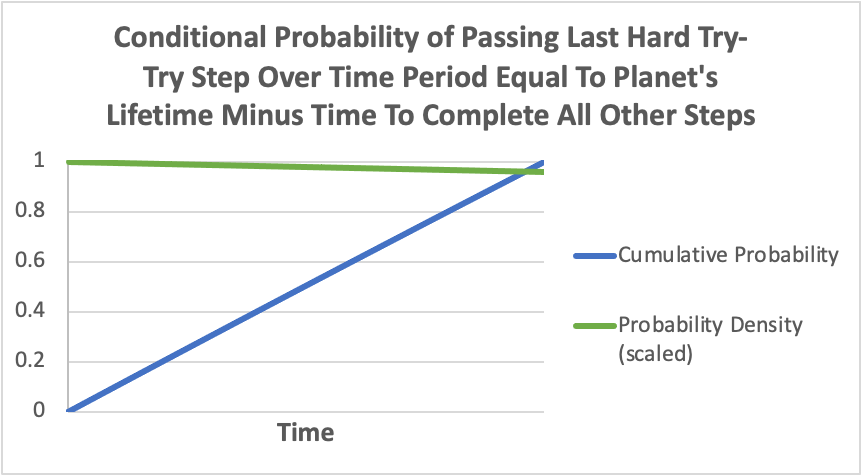
If at least one of the steps is a hard step, and conditional on passing all the steps with Σti < T, then the expected remaining time after the entire sequence has been completed, E(T - Σti | Σti < T), would be equal to the expected time that the last hard step took to complete. This is, again, because this hard step would face a uniform distribution for it’s time to completion within the window of interest, and the mean value of a uniform distribution would be halfway.
This result might not be immediately obvious if this step is not the last step (ie., if the last step is instead an easy step), but there are two ways to see that this doesn’t matter.
First, while in reality the steps may have a specific order (eg., it’s impossible for a form of multicellular life to evolve higher-level reasoning, communication, etc, before multicellular life evolves at all), in the simple mathematical model we’re considering, the order doesn’t matter; all that matters is that t1 + t2 + t3 + … + tn ≤ T. If we were to switch two steps, say s1 and s2, then we are instead left with the condition t2 + t1 + t3 + … + tn ≤ T, which is the same thing. So if the last step is not a hard step, we can simply conceptually switch the order of the steps such that the last step is a hard step. (It should also be clear that any of the hard steps could be switched to last, in which case each of their expected time would equal the expected remaining time – and that of each other). Second, if there are easy step(s) remaining after the last hard step, and if the hard step takes until the very end of the window of remaining time, then there might not be enough time to complete these easy step(s). So the existence of easy steps after the last hard step would “eat into” the end of the viable window for this last hard step to complete, and we’d again be left with, in expectation (conditional on completing the sequence), half of the remaining time (minus what will be eaten into by the easy step(s)) for the last hard step, and the other half for the time remaining after the entire sequence.
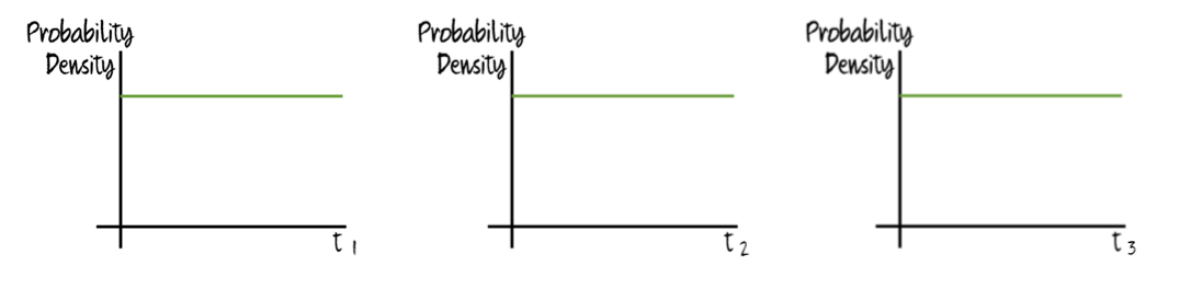
With multiple hard steps, these hard steps would all take the same expected time (conditional on completing the sequence). First, this is due to the reasoning from the above paragraph (that each could be switched to be “last” and thus equal in expectation to the remaining time after all the steps are completed), and also because, again, these hard steps will all face the same distribution for time to completion (a uniform distribution) within the time window of interest (time ≤ T), so they will all have the same expected value (and the same expected value given constraint Σti ≤ T).
So we are left with, conditional on the sequence being completed, the easy step(s) eating into the time window, and the rest of the time in the window being split evenly (in expectation) between each of the hard steps and also the time remaining after completing the entire sequence.
A couple points of clarification
First, none of the logic of the above is specific to either intelligence or intergalactic civilization. If any other development requires a sequence of steps that follow the same try-try dynamics and must all be passed in some time window, then the same logic applies.
For instance, consider the sequence of steps required for the development of a large, complex, multicellular lifeform capable of surviving in lava. Such a sequence would presumably start off looking similar to that for an intelligent, technological lifeform, but then would diverge. Such a sequence (after the formation of a habitable celestial body) may be something like: biomolecules -> simple cells -> complex cells -> evolutionary meta-improvement -> multicellularity -> diversification & complexity -> evolution of adaptations to survive in lava. If we assume these steps can be modeled as try-try steps, and if we condition on planets that have just completed this sequence, then on each of these planets, we would expect that the hard steps within this sequence would have taken the same expected time, and this would also be the expected remaining time for the habitability of the planet.
Due to anthropic reasoning, we may assume that there’s greater reason to believe there were hard steps along the path to humans than along observed paths to other things, but this point doesn’t affect the overarching logic of how a try-try step model should work.
A second point of clarification is needed around the habitability window, T. If passing a step would change the habitability window, this change in the habitability window should not be considered for how long that step would be expected to take (if passing a previous step would change the habitability window, however, that would affect the expected time that future completed hard steps take). This point can be seen from the logic of why we expect a completed hard try-try step to take half the remaining time – the probability density is flat over this time window. But if the window changes after the step is completed, that change can’t percolate backwards in time to change the amount of time the step had to be attempted.
The implication of this point is that, while longer time remaining in Earth’s habitability would imply, ceteris paribus, that the expected hard-step time was longer and thus that we had passed fewer hard steps already, while shorter remaining habitability would imply the opposite, we must be careful to use the remaining habitability from now had humans (and other intelligent, technological life) not evolved. If humans annihilate all life on Earth soon, or extend the habitability of Earth/civilization using advanced technology, none of this should be factored into the expected hard-step time or the number of hard steps we’ve already passed.
Limitations of this model, and implications of expansions
This model is obviously limited in several ways, but now that we understand the reasoning behind the model on a conceptual level, we can intuit what the effects would be from various changes or expansions.
As a recap, given hard try-try steps, they will all see ~flat probability density functions within the time window of interest, implying that (conditional on passing a sequence of steps) these hard steps will see the same expected time to complete as the expected remaining time, and since they will all see the same probability density functions within the time window of interest as each other, they will all see the same expected time to complete as each other.
What if we add steps that aren’t try-try steps or try-once steps? Perhaps some steps are slow, physics-limited steps and, while reliably passed within some time period, are very unlikely to be passed sooner (it has been suggested that the oxygenation of the atmosphere is one such step). Such steps aren’t well modeled by continuously rolling a die, but instead by a fuse that slowly burns down (and henceforth will be referred to as “fuse steps”). Such steps would have probability density functions that look like this:
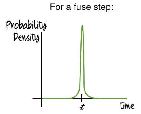
and would have characteristic times to pass, 𝓽j. Like easy try-try steps, fuse steps will simply eat into the window for the hard try-try steps (and the time remaining). Thus, if a sequence of i hard try-try steps and j fuse steps was passed on a planet with habitability window T (and where Σ𝓽j < T), then the expected time for each of the hard steps and the remaining time are all: (T - Σ𝓽j)/(i + 1).
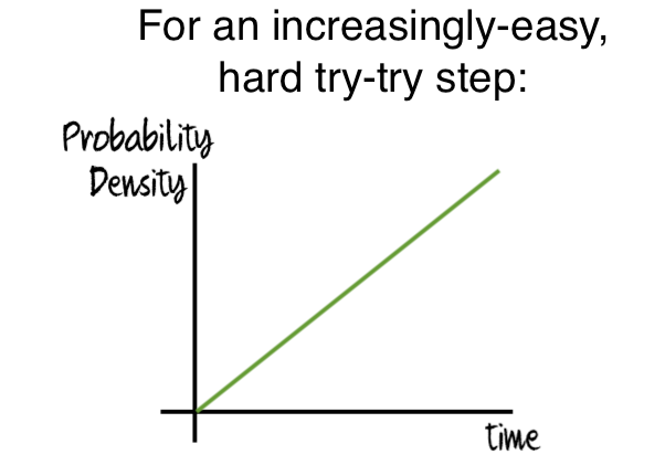
What if we modify the dynamics of try-try steps? Perhaps some try-try steps become easier to pass over time (for instance, the evolution of a lifeform with intelligence, cooperation, etc may have become more likely as brains grew and as biodiversity – and thus environmental complexity – increased). If such a step is a hard step, its probability density function over the time window of interest would look something like this:
If a sequence of hard try-try steps included one such increasingly easy step, as follows:
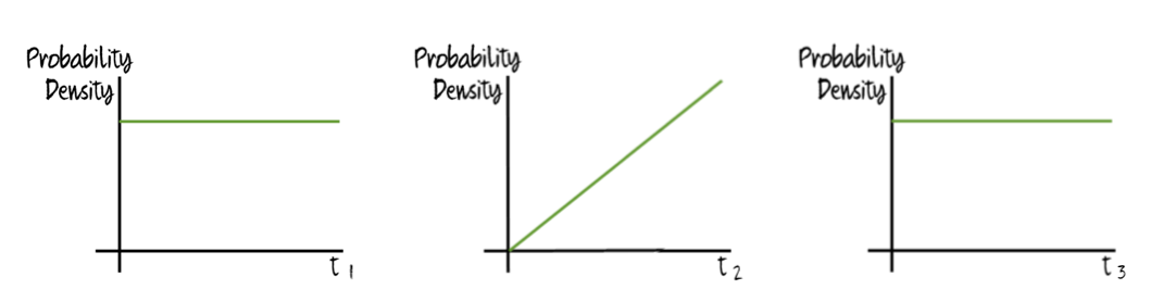
then (conditional on passing the sequence) the increasingly easy step would take in expectation longer than the other steps, as such a step has more probability mass on being passed later than earlier. The expected time remaining at the end would still be equal to the expected time for all the other hard steps.
If a step becomes increasingly difficult over time, then we’d expect the opposite result. Here, the longer we wait, the lower chances of passing it, so conditional on passing it, we’d expect to pass it relatively early (and the expected time remaining would still be equal to the expected time to pass each of the other hard steps).
We also get similar results if a hard try-try step doesn’t per se get easier or harder over time, but if attempting the step has a continual chance of creating a dead end. For instance, if, hypothetically, simple cells had some chance of destabilizing the climate and thus ending Earth’s habitability (while, again hypothetically, the arrival of complex cells ended this risk), then (assuming this is a hard step) the probability density of progressing from simple cells to complex cells would look like this:
as worlds in which the climate was destabilized would not be able to continue on to complex cells. If a sequence including this step was passed:
then we’d expect that step to have been passed earlier than the expected time for the other hard steps to be passed. If, on the other hand, all the hard steps faced the same constant (non-negligible) risk of annihilation (say, because of a constant risk that a nearby supernova would destroy all life on the planet), then the probability density of the various hard steps would look like this:
In this situation, because the hard steps would face the same probability density functions as each other, they would all take the same expected time (conditional on passing the sequence). However, these steps would still be frontloaded in their probabilities, so the expected remaining time after passing the sequence would be larger than the expected time to pass each of the steps.
Further expansions of the model could allow for greater nuance – such as “medium difficulty” steps with a 𝜏 similar to T, try-try steps that can only be passed in a narrow time window, multiple possible sequences to get from A to B, interdependencies between steps, and so on. I leave deriving the implications from these and other expansions of the model as an exercise for the reader.
7 comments
Comments sorted by top scores.
comment by Thomas Sepulchre · 2021-11-04T14:23:04.362Z · LW(p) · GW(p)
I feel like you are barking up the wrong tree. You are modelling the expected time needed for a sequence of steps, given the number of hard steps in the sequence, and given that all steps will be done before time T. I agree with you that those results are surprising, especially the fact that the expected time required for hard steps is almost independent from how hard those steps are, but I don't think this is the kind of question that comes to mind on this topic. The questions would be closer to
- How many hard steps has life on earth already achieved, and how hard were they?
- How many hard steps remain in front of us, and how hard are they?
- How long will it take us to achieve them / how likely is it that we will achieve them?
I may have misunderstood your point, if so, feel free to correct me.
Replies from: Daniel_Eth↑ comment by Daniel_Eth · 2021-11-05T21:39:21.669Z · LW(p) · GW(p)
Having a model for the dynamics at play is valuable for making progress on further questions. For instance, knowing that the expected hard-step time is ~identical to the expected remaining time gives us reason to expect that the number of hard steps passed on Earth already is perhaps ~4.5 (given that the remaining time in Earth's habitability window appears to be ~1 billion years). Admittedly, this is a weak update, and there are caveats here, but it's not nothing.
Additionally, the fact that the expected time for hard steps is ~independent of the difficulty of those steps tells us that, among other things, the fact that abiogenesis was early in Earth's history (perhaps ~400 MY after Earth formed) is not good evidence that abiogenesis is easy, as this is arguably around what we'd expect from the hard-step model (astrobiologists have previously argued that early abiogenesis on Earth is strong evidence for life being easy and thus common in the universe, and that if it was hard/rare that we'd expect abiogenesis to have occurred around halfway through Earth's lifetime).
Of course, this model doesn't help solve the latter two questions you raised, as it doesn't touch on future steps. A separate line of research that made progress on those questions (or a different angle of attack on the questions that this model can address) would also be a valuable contribution to the field.
Replies from: Thomas Sepulchre↑ comment by Thomas Sepulchre · 2021-11-08T15:19:09.807Z · LW(p) · GW(p)
Sorry for this late response
For instance, knowing that the expected hard-step time is ~identical to the expected remaining time gives us reason to expect that the number of hard steps passed on Earth already is perhaps ~4.5 (given that the remaining time in Earth's habitability window appears to be ~1 billion years).
I actually disagree with this statement. Assuming from now on that , so that we can normalize everything, your post shows that, if there are hard steps, given that they are all achieved, then the expected time required to achieve all of them is . Thus, you have built an estimator of , given : .
Now you want to solve the reverse problem: there is hard steps, and you want to estimate this quantity. We have one piece of information, which is . Therefore, the problem is, given , to build an estimator . This is not the same problem. You propose to use . The intuition, I assume, is that this is the inverse function of the previous estimator.
The first thing we could expect from this estimator is to have the correct expected value, i.e. . Let's check that.
The density of is (quick sanity check here : the expected value of is indeed ). From this we can derive the expected value . And we conclude that
How did this happen? Well, it happened because it is likely for to be really close to 1, which makes explode.
Ok, so the expected value doesn't match anything. But maybe is the most likely result, which would already be great. Let's check that too.
The density of is . Since , we have , therefore . We can derive this to get the argmax :, and therefore . Surprisingly enough, the most likely result is not
Just to be clear about what this means, if there are infinitely many planets in the universe on which live sentient species as advanced as us, and on each of them a smart individual is using your estimator to guess how many hard step they already went through, then the average of these estimates is infinite, and the most common result is .
Fixing the estimator
An easy thing is to find the maximum likelihood estimator. Just use and, if you check the math again, you will see that the most likely result is . Matching the expected value is a bit more difficult, because as soon as your estimator looks like , the expected value will be infinite.
For us, , therefore the maximum likelihood estimator gives us . Therefore, 10 hard steps seems a more reasonable estimate than 4.5
Replies from: Daniel_Eth↑ comment by Daniel_Eth · 2021-11-08T22:37:27.209Z · LW(p) · GW(p)
The intuition, I assume, is that this is the inverse function of the previous estimator.
So the estimate for the number of hard steps doesn't make sense in the absence of some prior. Starting with a prior distribution for the likelihood of the number of hard steps, and applying bayes rule based on the time passed and remaining, we will update towards more mass on k = t/(T–t) (basically, we go from P( t | k) to P( k | t)).
By "gives us reason to expect" I didn't mean "this will be the expected value", but instead "we should update in this direction".
↑ comment by Thomas Sepulchre · 2021-11-09T13:05:01.167Z · LW(p) · GW(p)
So the estimate for the number of hard steps doesn't make sense in the absence of some prior. Starting with a prior distribution for the likelihood of the number of hard steps, and applying bayes rule based on the time passed and remaining, we will update towards more mass on k = t/(T–t) (basically, we go from P( t | k) to P( k | t)).
Ok let's do this. Since is an integer, I guess our prior should be a sequence . We already know . We can derive from this , and finally . In our case,
I guess the most natural prior would be the uniform prior: we fix an integer , and set for . From this we can derive the posterior distribution. This is a bit tedious to do by hand, but easy to code. From the posterior distribution we can for example extract the expected value of : . I computed it for and voilà!

Obviously is strictly increasing. It also converges toward 10. Actually, for almost all values of , the expected value is very close to 10. To give a criterion, for , the expected value is already above 7.25, which implies that it is closer to 10 than to 4.5.
We can use different types of prior. I also tried (with a normalization constant), which is basically a smoother version of the previous one. Instead of stating with certainty "the number of hard steps is at most ", it's more "the number of hard steps is typically , but any huge number is possible". This gives basically the same result, except is separates from 4.5 even faster, as soon as .
My point is not to say that the number of hard steps is 10 in our case. Obviously I cannot know that. Whatever prior we may choose, we will end up with a distribution of probability, not a nice clear answer. My point is that if, for the sake of simplicity, we choose to only remember one number / to only share one number, it should probably not be 4.5 (or ), but instead 10 (or ). I bet that, if you actually have a prior, and actually make the bayesian update, you'll find the same result.
Replies from: Daniel_Eth↑ comment by Daniel_Eth · 2021-11-10T10:12:16.979Z · LW(p) · GW(p)
So again, I wasn't referring to the expected value of the number of steps, but instead how we should update after learning about the time – that is, I wasn't talking about but instead for various .
Let's dig into this. From Bayes, we have: . As you say, ~ kt^(k-1). We have the pesky term, but we can note that for any value of , this will yield a constant, so we can discard it and recognize that now we don't get a value for the update, but instead just a relative value (we can't say how large the update is at any individual , but we can compare the updates for different ). We are now left with ~ kt^(k-1), holding constant. Using the empirical value on Earth of , we get ~ k*0.82^(k-1).
If we graph this, we get:
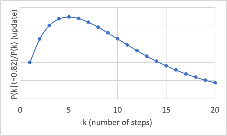
which apparently has its maximum at 5. That is, whatever the expected value for the number of steps is after considering the time, if we do update on the time, the largest update is in favor of there having been 5 steps. Compared to other plausible numbers for , the update is weak, though – this partiuclar piece of evidence is a <2x update on there having been 5 steps compared to there having been 2 steps or 10 steps; the relative update for 5 steps is only even ~5x the size of the update for 20 steps.
Considering the general case (where we don't know ), we can find the maximum of the update by setting the derivative of kt^(k-1) equal to zero. This derivative is (k ln(t) + 1)t^(k-1), and so we need , or . If we replace with , such that corresponds to the naive number of steps as I was calculating before, then that's . Here's what we get if we graph that:
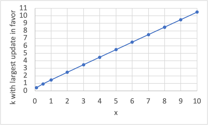
This is almost exactly my original guess (though weirdly, ~all values for are ~0.5 higher than the corresponding values of ).
Replies from: Thomas Sepulchre↑ comment by Thomas Sepulchre · 2021-11-10T14:43:06.451Z · LW(p) · GW(p)
I agree with those computations/results. Thank you