Recent Progress in the Theory of Neural Networks

post by interstice · 2019-12-04T23:11:32.178Z · LW · GW · 9 comments

Contents

  Infinite Width Nets: Initialization  
  Infinite Width: Training
  Significance and Limitations of Infinite-Width Limit  
   Generalization Theory 
  Relevance for Alignment  
None
9 comments

It's common wisdom that neural networks are basically "matrix multiplications that nobody understands" , impenetrable to theoretical analysis, which have achieved great results largely through trial-and-error. While this may have been true in the past, recently there has been significant progress towards developing a theoretical understanding of neural networks. Most notably, we have obtained an arguably complete understanding of network initialization and training dynamics in a certain infinite-width limit. There has also been some progress towards understanding their generalization behavior. In this post I will review some of this recent progress and discuss the potential relevance to AI alignment.

Infinite Width Nets: Initialization

The most exciting recent developments in the theory of neural networks have focused the infinite-width limit. We consider neural networks where the number of neurons in all hidden layers are increased to infinity. Typically we consider networks with a Gaussian-initialized weights, and scale the variance at initialization as $\frac{1}{\sqrt{H}}$, where $H$ is the number of hidden units in the preceding layer(this is needed to avoid inputs blowing up, and is also the initialization scheme usually used in real networks). In this limit, we have obtained an essentially complete understanding of both behavior at initialization and training dynamics[1]. (Those with limited interest/knowledge of math may wish to "Significance and Limitations" below).

We've actually had a pretty good understanding of the behavior of infinite-width neural networks at initialization for a while, since the work of Radford Neal(1994). He proved that in this limit, fully-connected neural networks with Gaussian-distributed weights and biases limit to what are known as Gaussian processes. Gaussian processes can be thought of the generalization of Gaussian distributions from finite-dimensional spaces to spaces of functions. Neal's paper provides a very clear derivation of this behavior, but I'll explain it briefly here.

A neural network with m real-valued inputs and 1 real valued outputs defines a function from $R^m$ to $R$. Thus, a distribution over the weights and biases of such a neural network -- such as the standard Gaussian initialization -- implicitly defines a distribution over functions on $R^m$. Neal's paper shows that, for fully-connected neural networks, this distribution limits to a Gaussian process.

What is a Gaussian process? It's a distribution over functions$f$ with the property that, for any finite collection of points $X_1,...,X_N$, the values$f\left(X_1\right),...,f\left(X_N\right)$ have a joint distribution which is a multivariate Gaussian. Any Gaussian process is uniquely defined by its mean and covariance functions, $\mu \left(x\right)$ and $C(x,x^{\prime })$. For points $X_1,...,X_N$, the distribution of $f\left(X_1\right),...,f\left(X_N\right)$ will have mean $\mu \left(X_1\right),...,\mu \left(X_N\right)$ with covariance matrix $C_{ij}=C(X_i,X_j)$.

The argument that fully-connected neural networks limit to Gaussian processes in the infinite-width limit is pretty simple. Consider a three-layer neural network, with an activation function $\sigma$ in the second layer and a single linear output unit. This network can be defined by the equation $y=\sum V^k\sigma (\sum W^{kj}{X}^j)$ . At initialization, $V$ and $W$ are filled with independent Gaussians, with variance of $V$ scaled as the inverse square-root of the number of hidden-units.

Each hidden unit $h^k$ will has a value for each of the inputs $X_i$ , $h^k\left(X_i\right)=\sigma (\sum W^{kj}{X}_i^j)$. Since $W$ is random, for each $k$, $h^k\left(\overrightarrow{X}\right)$ is an independent random vector(where we write $\overrightarrow{X}$ for $X_1,...,X_N$). All of these random vectors follow the same distribution, and the output $\overrightarrow{y}=f\left(\overrightarrow{X}\right)$ of the network is simply the sum of these identical distributions multiplied by the univariate Gaussians $V^k$. By the multidimensional central limit theorem, this sum will tend to a multidimensional Gaussian.

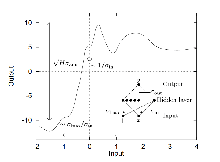
Image: a sample from a GP defined by a neural net. From McKay(1995).

Extending this argument to multiple hidden layers is also pretty easy. By induction, the pre-activations of each unit in hidden layer J have identical Gaussian process distributions, which induces identical(non-Gaussian,generically) joint distributions on the activations. The pre-activations of layer J+1 are the sum of these activations multiplied by univariate Gaussians, hence the central limit theorem can be applied again to show that these pre-activations have a joint Gaussian distribution for any set of inputs, hence they have a Gaussian process distribution. This inductive process can be used to compute the mean $\mu \left(\overrightarrow{X}\right)$ and covariance $C(\overrightarrow{X},\overrightarrow{X})$ of the output to an arbitrary depth for a given set of inputs $\overrightarrow{X}$. For many activation functions including ReLUs, this computation can be done exactly, giving an explicit expression for the distribution over outputs at initialization.

More recently, this behavior was proved to extend to CNNs, and then pretty much all classes of neural network architecture currently used. In convolutional neural nets, the infinite 'width' limit is taken with respect to the number of filters.

Infinite Width: Training

Okay, so we can understand how neural nets behave at initialization in this limit. But we don't care that much about initialization -- what really matters is what function it represents after the training process is over. The training process is over a complex, non-linear space, and seems much less tractable to the kind of analysis used at initialization. Surprisingly, however, there is a similar simplification that occurs when we pass to the infinite-width limit. For those of you who know some machine learning, it turns out that, in this limit, neural networks behave as a kind of kernel machine, using the so-called neural tangent kernel(NTK).

In this case, the derivation of the infinite-width behavior is more complex, so I'll just explain what that behavior is. The key is to consider the effect of the training process on the values $f\left(X_1\right),...,f\left(X_N\right)$ at the points to be classified, rather than the weights of the network. Consider two inputs $X_1,X_2$. Imagine taking a step of gradient descent on the network weights $\theta$ to adjust the network output $f\left(X_1\right)$. What will the effect of this be on $f\left(X_2\right)$? To first order, a given change in the weights $\Delta \theta$ will change $f\left(X_2\right)$ by $<{\nabla }_{\theta }f\left(X_2\right),\Delta \theta >$. Taking a gradient step in the direction of $f\left(X_1\right)$ will cause a change in the weights of ${\nabla }_{\theta }f\left(X_1\right)$. Therefore, taking a step of gradient descent at $f\left(X_1\right)$ will have the effect of changing $f\left(X_2\right)$ by $<{\nabla }_{\theta }f\left(X_1\right),{\nabla }_{\theta }f\left(X_2\right)>$ We can construct an $N\times N$ matrix $K_{\theta }$ with entries $K_{\theta ,i,j}=<{\nabla }_{\theta }f\left(X_i\right),{\nabla }_{\theta }f\left(X_j\right)>$ Taking a step of full-batch gradient descent in the direction $\overrightarrow{\Delta }$ (indexed along $\overrightarrow{X}$) will, to first order, effect a change in the outputs of $K_{\theta }\overrightarrow{\Delta }$.

Of course, this doesn't really simplify things much, as the matrix $K_{\theta }$ is itself dependent on the weights, which vary both randomly at initialization and during training. The insight of the NTK paper is that in the infinite-width limit, this dependence disappears. For infinite-width networks:

i) at initialization, $K_{\theta }$ becomes a deterministic matrix $K_{\infty }$

ii) during training, $K_{\infty }$ doesn't change. (The weights still change during training, but their change is small enough that $K_{\infty }$ is unaffected)

Therefore, training on a set of N inputs can be perfectly simulated by just calculating $K_{\infty }$ for those inputs, then using $K_{\infty }$ to iterate the training(in practice, the end result of training is instead calculated directly, which can be done by inverting $K_{\infty }$) An inductive formula for calculating $K_{\infty }$ is given in the NTK paper.

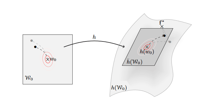
Another way of thinking about the NTK is that it is essentially equivalent to taking the first-order Taylor expansion of a neural network about its initial parameters. In this regime, the response of the output to changes in the parameters is linear(though the output is not linear in the network input!) Then the above papers prove that, in the infinite-width limit, the training trajectory stays close to that of its Taylor expansion.

Image: The network's training trajectory stays close to that of its linearization $\overline{h}$ . From Chizat&Bach(2018).

The NTK was originally defined for simply-connected models, but was later extended to convolutional nets, and now pretty much all network architectures. (As a historical note, many of the ideas behind the NTK were discovered before the paper coining the term NTK, check out this paper for instance)

For those of you wanting to attain a deeper understanding, the original NTK paper is a pretty clear read, as is this blog post.

Significance and Limitations of Infinite-Width Limit

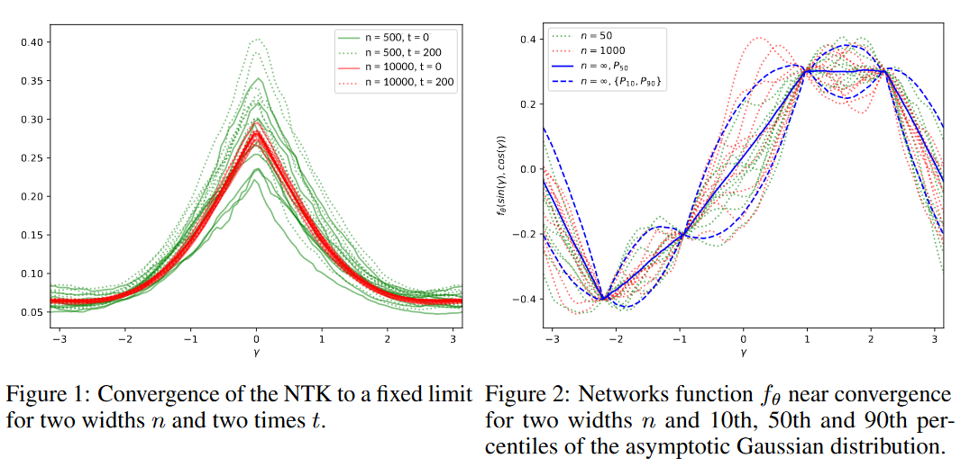
So what's the upshot of all this? Does studying the infinite-width limit tell us anything about the success of finite neural networks? I'd argue that it does. Several of the papers above include comparisons between the output of finite-width networks and the analytically-computed predictions of the associated Gaussian processes and neural tangent kernel. Agreement was often pretty close:

Image: convergence of NTK for one-dimensional input space. From the NTK paper.

Moreover, the performance of the NTK-based methods on learning tasks was impressive. This paper used the kernel associated with deep CNN to classify CIFAR-10 images, achieving 77% accuracy, a new record for kernel-based methods. This is only 6% lower than the performance of the original network. The kernel-like behavior of neural networks may not account for all of their good performance, but it seems to explain at least some of it.

Ultimately, the point of relating neural networks to kernel methods is that kernel methods are much simpler. Kernel methods are a sort of generalization of linear models, in which inputs are projected into a higher-dimensional space where they can be linearly separated. Kernels are tractable to mathematical analysis. It's possible to prove that kernel methods will always converge to a global minimum (on the training points) under gradient descent, and thus prove that neural networks will always converge to a minimum when they have enough hidden units. Another mathematical tool for analyzing kernels is their eigen-decomposition: see for instance this paper which finds that the NTK is diagonalized in the Fourier basis on the binary cube. They then use the eigenvalue associated to various functions as a measure of complexity, finding that it correlates well with the generalization performance of the neural network when learning that function.

Despite this, there are limitations to kernel-based analysis. A given NTK will usually underperform its associated neural network, and as far as I know nobody has even tried to apply NTK methods to problems such as ImageNet. (mostly due to computational costs, as using the NTK for regression scales like $N^3$ in number of data points). There are theoretical works that suggest that there exist problems solvable by neural networks which no kernel-based method can solve. See also this paper on the limits of the 'lazy regime', their term for training regimes in which classifiers are approximately linear in their parameters(which includes the infinite-width limit).

Generalization Theory

The works above on the infinite-width limit explain, to some extent, the success of SGD at optimizing neural nets, because of the approximately linear nature of their parameter-space. A remaining piece of the puzzle is generalization, explaining why the global minimum found on the training set will tend to work well on new data points.

Traditionally, statistical learning theory has focused on classes of models where there number of potential functions learnable by that class is small. However, neural networks are usually capable of fitting arbitrary functions of their dataset, so many tools used to prove that models have low generalization error have failed: the bounds they give are vacuous, meaning that they can't certify that the model will perform better than random guessing. This issue was popularized in a 2017 paper by Zhang et al.

Despite this, recently some non-vacuous generalization bounds have been proven. Thus far, the only non-vacuous bounds for 'real' datasets such as MNIST have used PAC-Bayes methods. These methods replace an individual neural net with a learned distribution over network parameters, and introduce a fixed prior over the parameters. The generalization error is bounded by (the square root of) the KL divergence between the prior distribution and the learned distribution. Intuitively: a low KL divergence means the learned distribution has a short description length w.r.t. the prior, and there are only so many such distributions(sort of), so one of them matching the training inputs would be unlikely unless it truly captured part of the underlying function. PAC-Bayes bounds cannot guarantee high performance off the training set, but they can provably bound the error with high probability, assuming that the training data has been fairly sampled from the underlying distribution.

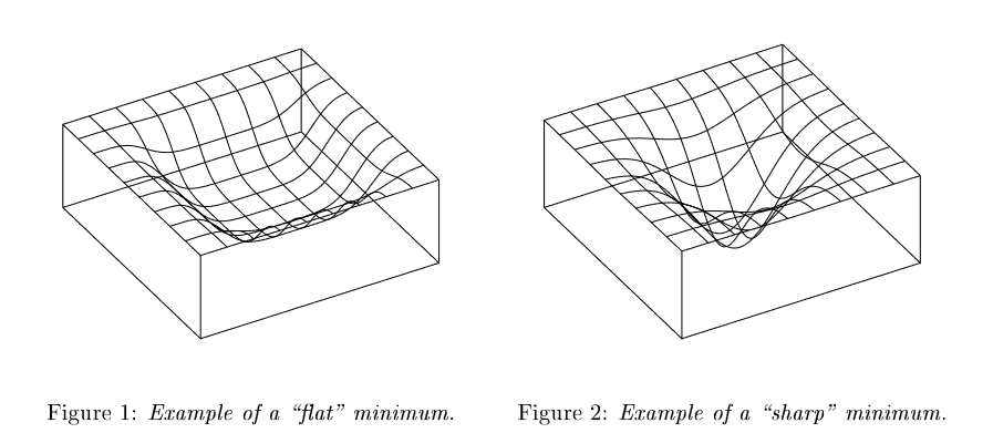
The first work to use PAC-Bayes bounds for modern neural networks was written by Dziugaite&Roy. They were able to prove non-vacuous bounds on a binarized version of MNIST -- not as trivial as it sounds, given that the classifying networks had hundreds of thousand of parameters. Taking as their prior a Gaussian distribution centered at initialization, the authors represented the learned network with another Gaussian distribution whose parameters they optimized with SGD to minimize the PAC-Bayes bound on total error. This work was inspired by the notion of flat minima, which is the idea that gradient descent is biased toward wide minima in parameter space, where perturbing the parameters does not affect the loss much. From a minimum description length principle, flat minima can be described using fewer bits because of their width, which should imply that solutions found by SGD have good generalization performance. The 'nonvacuous bounds' paper used a formalism inspired by this notion to derive provable generalization bounds.

Image: flat vs. sharp minima. From Hochreiter&Schmidhuber(1996).

A later paper made the connection between PAC-Bayes bounds and compression more explicit. They used techniques for compressing the parameters of a neural network to store networks solving full MNIST and ImageNet using far fewer bits than their original size. Using a PAC-Bayes prior over code-words, they were able to provably verify at least 54% accuracy on MNIST and at least 3.5% accuracy on ImageNet(non-trivial given the huge number of classes in ImageNet).

Deriving bounds on the generalization error might seem pointless when it's easy to do this by just holding out a validation set. I think the main value is in providing a test of purported theories: your 'explanation' for why neural networks generalize ought to be able to produce non-trivial bounds on their generalization error.

Relevance for Alignment

At this stage, theoretical research on neural networks is not yet directly useful for alignment. Its goal is more conceptual clarity than producing tools that would be useful for practitioners, or even theoretical insights that are directly relevant to alignment-type issues.

In the long run, though, I believe that this sort of research could be crucial for creating aligned AI. It seems plausible that neural networks will be used to build AGI, or be a major component of AGI. If that happens, deeply understanding the implicit bias and optimization properties of these networks will be extremely important for a variety of purposes from choosing the class of models to enabling ongoing monitoring of what they have learned. This sort of theoretical understanding will likely be essentially in the implementation of alignment schemes such as IDA, and could enable more powerful versions of existing transparency [AF · GW]and robustness methods.

But even if you think, as MIRI does(?), that neural networks are ultimately too insecure to build aligned AI, I believe trying to understand neural networks is still a worthwhile goal. Neural networks are one of the only techniques we have with anything approaching the generality needed for AGI. If alignment researchers want to build a 'secure version' of neural networks, then it seems necessary to first understand what factors contribute to their strong performance. Then it may be possible to isolate those factors in a more secure and transparent class of models. In contrast, attempting to derive such a class of models from pure thought, or experiments isolated from the mainstream of ML, seems much more difficult. Almost no AI techniques people think of work very well, so the existence of one that does seem to work well on a variety of realistic problems is a powerful and hard-won clue.

The upshot of this for how people interested in alignment should spend their time and money isn't as clear. This seems like an area that academia and industry is already pretty interested in and successful at studying. At the same time, I think there is still a huge amount of work to do and lots of stuff we don't understand, so I could imagine marginal researchers being useful. At the very least, I think it would be a good thing if alignment researchers were aware that advances in the theory of neural networks are happening, and kept tabs on new developments.

Footnotes

[1]: Technical note: Taking the limit of all layers to infinity is ambiguous; do you take the first layer to infinity, then the second, etc., or do you take them all to infinity at once? It turns out you get the same answer either way, so I'll just present as if taking the limits sequentially.

9 comments

Comments sorted by top scores.